Model Diagnostics and Comparison • uncounted

This vignette demonstrates the diagnostic and model-comparison tools available in the uncounted package. We cover goodness-of-fit statistics, residual analysis, rootograms, exploratory log-log plots, leave-one-out sensitivity analysis, and gamma profiling. Together these tools help you decide which model specification is most appropriate and whether the population-size estimates are robust.

1. Setup: fitting Poisson and Negative Binomial models

We use the irregular_migration dataset shipped with the package. Two models are fitted—Poisson and Negative Binomial—with year and sex covariates on alpha and year covariates on beta.

library(uncounted)
data(irregular_migration)

fit_po <- estimate_hidden_pop(
  data = irregular_migration,
  observed = ~ m, auxiliary = ~ n, reference_pop = ~ N,
  method = "poisson",
  cov_alpha = ~ factor(year) + sex, cov_beta = ~ factor(year),
  countries = ~ country_code
)

fit_nb <- estimate_hidden_pop(
  data = irregular_migration,
  observed = ~ m, auxiliary = ~ n, reference_pop = ~ N,
  method = "nb",
  cov_alpha = ~ factor(year) + sex, cov_beta = ~ factor(year),
  countries = ~ country_code
)

Quick summaries:

summary(fit_po)
#> Unauthorized population estimation
#> Method: POISSON | vcov: HC3 
#> N obs: 1382 
#> Gamma: 0.007255 (estimated) 
#> Log-likelihood: -8217.25 
#> AIC: 16462.49  BIC: 16535.73 
#> Deviance: 13831.69 
#> 
#> Coefficients:
#>                          Estimate Std. Error z value  Pr(>|z|)    
#> alpha:(Intercept)       0.7889384  0.0904971  8.7178 < 2.2e-16 ***
#> alpha:factor(year)2020  0.0013183  0.0961281  0.0137 0.9890579    
#> alpha:factor(year)2021 -0.0173547  0.0874282 -0.1985 0.8426521    
#> alpha:factor(year)2022 -0.0936745  0.1093813 -0.8564 0.3917748    
#> alpha:factor(year)2023 -0.1136248  0.1774180 -0.6404 0.5218896    
#> alpha:factor(year)2024 -0.1692210  0.1612687 -1.0493 0.2940349    
#> alpha:sexMale           0.0419896  0.0458891  0.9150 0.3601795    
#> beta:(Intercept)        0.6755335  0.1951985  3.4608 0.0005387 ***
#> beta:factor(year)2020   0.1890802  0.2277589  0.8302 0.4064387    
#> beta:factor(year)2021   0.2334479  0.2128471  1.0968 0.2727346    
#> beta:factor(year)2022   0.0887221  0.2489532  0.3564 0.7215557    
#> beta:factor(year)2023  -0.0522207  0.3786238 -0.1379 0.8903018    
#> beta:factor(year)2024  -0.3228057  0.3185915 -1.0132 0.3109513    
#> ---
#> Signif. codes:  0 '***' 0.001 '**' 0.01 '*' 0.05 '.' 0.1 ' ' 1
#> 
#> -----------------------
#> Population size estimation results:
#>   (BC = bias-corrected using model-based variance)
#>                       Observed Estimate Estimate (BC) CI lower CI upper
#> year=2019, sex=Female    1,535   21,124        21,093    3,394  131,073
#> year=2019, sex=Male      5,069   60,051        59,968   10,189  352,946
#> year=2020, sex=Female      698   23,658        23,593    6,025   92,387
#> year=2020, sex=Male      2,700   66,785        66,594   22,935  193,363
#> year=2021, sex=Female      483   22,783        22,718    7,267   71,020
#> year=2021, sex=Male      2,622   65,124        64,929   32,335  130,378
#> year=2022, sex=Female      317   14,118        14,082    2,477   80,072
#> year=2022, sex=Male      2,632   32,913        32,836    7,366  146,377
#> year=2023, sex=Female      523   12,074        12,053      533  272,376
#> year=2023, sex=Male      3,839   28,857        28,813    1,219  681,051
#> year=2024, sex=Female      956    7,107         7,101      577   87,449
#> year=2024, sex=Male      5,731   17,462        17,448    1,177  258,669
summary(fit_nb)
#> Unauthorized population estimation
#> Method: NB | vcov: HC1 
#> N obs: 1382 
#> Gamma: 0.020902 (estimated) 
#> Theta (NB dispersion): 1.3553 
#> Log-likelihood: -2621.12 
#> AIC: 5272.23  BIC: 5350.7 
#> Deviance: 1275.97 
#> 
#> Coefficients:
#>                         Estimate Std. Error z value  Pr(>|z|)    
#> alpha:(Intercept)       0.815797   0.034293 23.7889 < 2.2e-16 ***
#> alpha:factor(year)2020 -0.041875   0.057015 -0.7344 0.4626758    
#> alpha:factor(year)2021  0.075429   0.059616  1.2653 0.2057804    
#> alpha:factor(year)2022 -0.029911   0.073397 -0.4075 0.6836246    
#> alpha:factor(year)2023  0.015692   0.055918  0.2806 0.7789985    
#> alpha:factor(year)2024  0.069563   0.047739  1.4572 0.1450728    
#> alpha:sexMale           0.044291   0.013134  3.3721 0.0007459 ***
#> beta:(Intercept)        0.873222   0.092126  9.4786 < 2.2e-16 ***
#> beta:factor(year)2020   0.140642   0.116669  1.2055 0.2280191    
#> beta:factor(year)2021   0.468272   0.121552  3.8524 0.0001170 ***
#> beta:factor(year)2022   0.185329   0.151494  1.2233 0.2212012    
#> beta:factor(year)2023   0.184161   0.110429  1.6677 0.0953779 .  
#> beta:factor(year)2024   0.132660   0.092733  1.4306 0.1525565    
#> ---
#> Signif. codes:  0 '***' 0.001 '**' 0.01 '*' 0.05 '.' 0.1 ' ' 1
#> 
#> -----------------------
#> Population size estimation results:
#>   (BC = bias-corrected using model-based variance)
#>                       Observed Estimate Estimate (BC) CI lower CI upper
#> year=2019, sex=Female    1,535   27,920        25,603   12,669   51,744
#> year=2019, sex=Male      5,069   82,539        75,303   35,607  159,254
#> year=2020, sex=Female      698   19,970        18,074    6,728   48,554
#> year=2020, sex=Male      2,700   57,341        51,568   18,777  141,623
#> year=2021, sex=Female      483   82,856        72,726   24,247  218,134
#> year=2021, sex=Male      2,622  257,069       223,983   71,877  697,978
#> year=2022, sex=Female      317   38,116        34,521    7,934  150,206
#> year=2022, sex=Male      2,632   89,857        82,042   20,886  322,269
#> year=2023, sex=Female      523   66,725        60,793   20,297  182,084
#> year=2023, sex=Male      3,839  159,251       146,494   52,769  406,687
#> year=2024, sex=Female      956  120,658       110,946   46,472  264,872
#> year=2024, sex=Male      5,731  302,323       280,070  120,941  648,573

2. Model comparison

Comparison table

compare_models() produces a side-by-side table of log-likelihood, AIC, BIC, deviance, Pearson chi-squared, RMSE, and three pseudo $R^2$ measures:

R2_cor: $\mathrm{cor}(m, \hat\mu)^2$ — squared correlation between observed and fitted values.
R2_D: Explained deviance $1 - D(\text{model}) / D(\text{null})$ , where the null model is the same specification without covariates (single $\alpha$ , single $\beta$ ). Measures how much covariates improve the fit beyond the baseline power-law structure.
R2_CW: Cameron–Windmeijer (1996) pseudo $R^2$ , which uses the model-implied variance function $V(\mu)$ — specifically designed for count data regression.

Models are sorted by AIC (the default). Note that R2_D compares the fitted model against a null model (same method, no covariates). If the model has no cov_alpha / cov_beta, then R2_D = 0 by construction — it only becomes informative when covariates are present.

comp <- compare_models(Poisson = fit_po, NB = fit_nb, sort_by = "AIC")
comp
#> Model comparison
#> ------------------------------------------------------------ 
#>    Model  Method Constrained n_par   logLik      AIC      BIC Deviance
#>       NB      NB       FALSE    15 -2621.12  5272.23  5350.70  1275.97
#>  Poisson POISSON       FALSE    14 -8217.25 16462.49 16535.73 13831.69
#>  Pearson_X2   RMSE R2_cor    R2_D  R2_CW
#>     3090.80 205.92 0.4058 -0.0030 0.9526
#>    17500.68  52.53 0.8280  0.3139 0.9827

Lower AIC and BIC values indicate a better trade-off between fit and complexity. The Pearson chi-squared statistic divided by its degrees of freedom (approximately n_obs - n_par) gives a quick dispersion check: values much greater than 1 suggest overdispersion, which favours the NB model over Poisson.

Likelihood ratio test

Because the Poisson model is nested within the Negative Binomial (the Poisson is the NB with theta -> infinity), we can use a likelihood ratio test. lrtest() applies the boundary correction of Self & Liang (1987) automatically when comparing Poisson against NB, because the dispersion parameter lies on the boundary of the parameter space under H0.

lrtest(fit_po, fit_nb)
#> Likelihood ratio test
#> ---------------------------------------- 
#> Model 1: POISSON   (logLik = -8217.25 )
#> Model 2: NB   (logLik = -2621.12 )
#> LR statistic: 11192.26 on 1 df
#> (Boundary-corrected: 0.5 * P(chi2 > LR), Self & Liang 1987)
#> p-value: < 2.2e-16

A small p-value indicates significant overdispersion, favouring the NB model.

3. Residual diagnostics

Residual types

The residuals() method supports four types:

response: raw residuals, $m_i - \hat\mu_i$ .
pearson: standardised by the variance function, $(m_i - \hat\mu_i) / \sqrt{V(\hat\mu_i)}$ .
deviance: signed square root of individual deviance contributions.
anscombe: variance-stabilising residuals (approximately standard normal for a well-specified model).

r_resp <- residuals(fit_nb, type = "response")
r_pear <- residuals(fit_nb, type = "pearson")
r_dev  <- residuals(fit_nb, type = "deviance")
r_ansc <- residuals(fit_nb, type = "anscombe")

summary(r_pear)
#>     Min.  1st Qu.   Median     Mean  3rd Qu.     Max. 
#> -1.15137 -0.59480 -0.28872  0.03626  0.11100 22.91547
summary(r_ansc)
#>     Min.  1st Qu.   Median     Mean  3rd Qu.     Max. 
#> -24.1591  -1.0757  -0.4677  -0.3349   0.1768   9.4208

Four-panel diagnostic plot

plot() on a fitted model produces the Zhang (2008) four-panel display:

Fitted vs Observed (sqrt scale) – points should cluster around the 45-degree line.
Anscombe residuals vs fitted – the running mean should be flat near zero (no systematic misfit).
Scale-Location – absolute Anscombe residuals vs fitted; an increasing trend signals under-modelled variance.
Normal Q-Q – Anscombe residuals should follow the reference line if the distributional assumption holds.

op <- par(mfrow = c(2, 2))
plot(fit_nb, ask = FALSE)

par(op)

What to look for:

Curvature in Panel 1 suggests the mean function is misspecified.
A non-flat smoother in Panel 2 indicates systematic bias at certain fitted-value ranges.
A fan shape in Panel 3 points to overdispersion or heteroscedasticity.
Heavy tails or S-shapes in Panel 4 indicate departure from the assumed distribution.

Compare with the Poisson fit to see whether switching to NB resolves any patterns:

op <- par(mfrow = c(2, 2))
plot(fit_po, ask = FALSE)

par(op)

4. Rootograms

Rootograms (Kleiber & Zeileis, 2016) compare the observed and fitted count-frequency distributions directly. Three display styles are available:

hanging (default): observed bars are hung from the fitted curve. If the model fits well, the bottom of each bar touches zero.
standing: observed bars stand on the x-axis with the fitted curve overlaid. Harder to judge discrepancies visually.
suspended: plots the difference $\sqrt{f_\text{obs}} - \sqrt{f_\text{exp}}$ directly. Bars crossing zero indicate over- or under-prediction at that count.

rootogram(fit_nb, style = "hanging")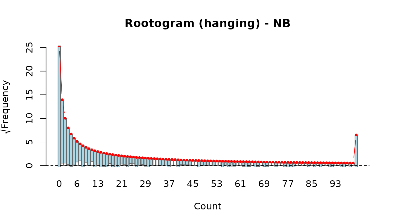

rootogram(fit_po, style = "hanging")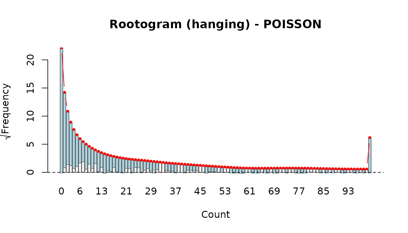

Compare the two: if the Poisson rootogram shows bars consistently hanging below the zero line at small counts and above at moderate counts, this is a classic overdispersion signature that the NB model should correct.

rootogram(fit_nb, style = "standing")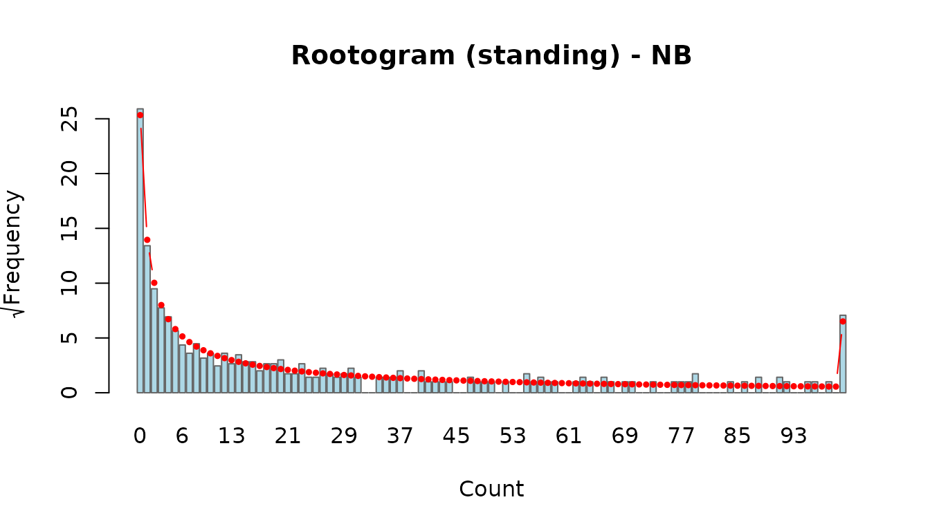

rootogram(fit_nb, style = "suspended")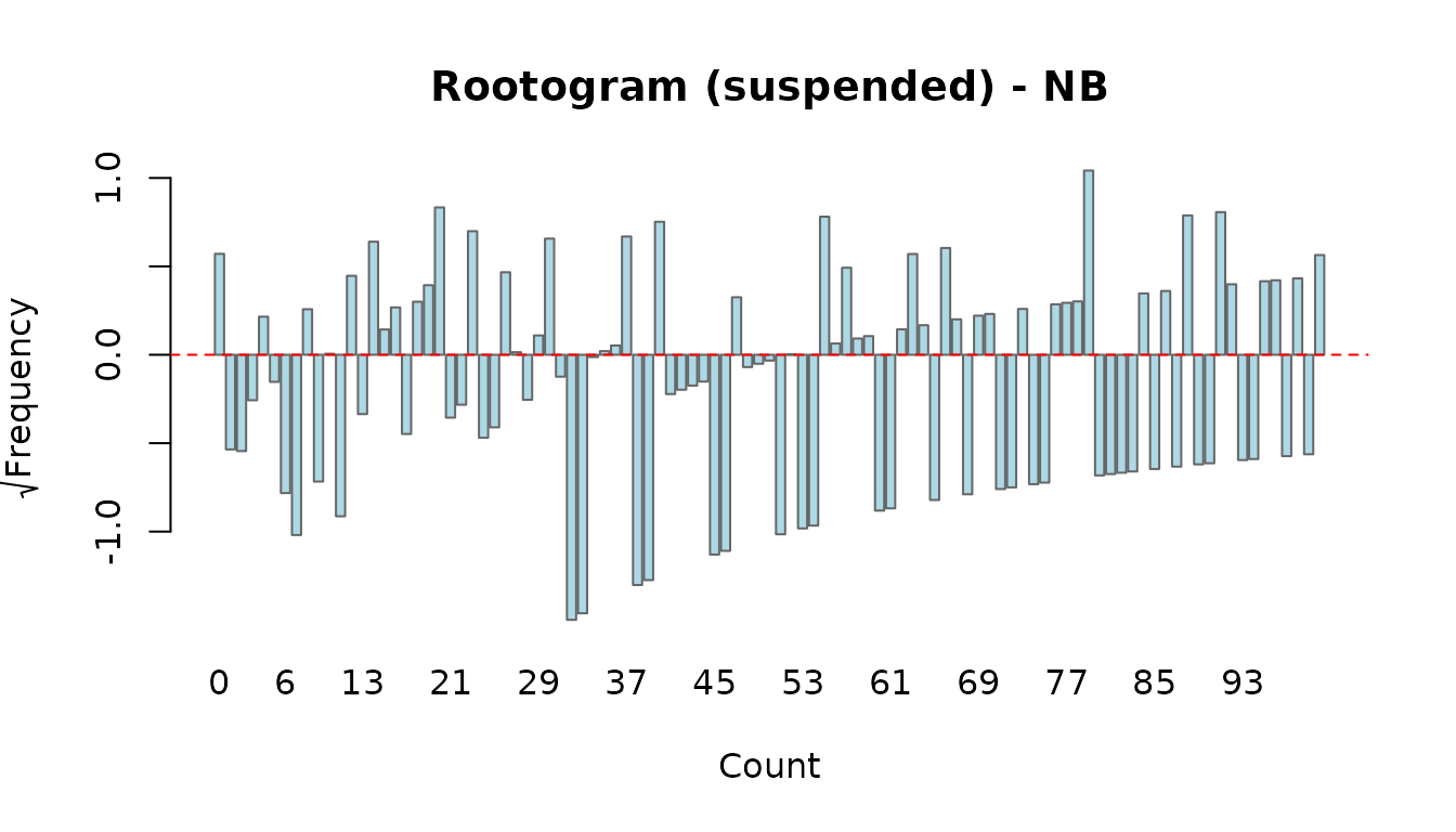

5. Exploratory log-log plots

Before or after fitting, plot_explore() produces two log-log scatter plots that reveal the marginal relationships underlying the power-law model:

log(m/N) vs log(N): the slope approximates $\alpha - 1$ . A slope near zero means the apprehension rate is roughly independent of population size ( $\alpha \approx 1$ ). A negative slope indicates decreasing returns to scale ( $\alpha < 1$ ).
log(m/N) vs log(n/N): the slope approximates $\beta$ . A positive slope confirms that the auxiliary rate is predictive of the apprehension rate.

Observations with $m = 0$ or $n = 0$ are excluded (undefined on the log scale).

plot_explore(fit_nb)

These plots are exploratory visual checks. The OLS lines overlaid are rough guides—the formal model accounts for covariates and the gamma offset.

6. Leave-one-out sensitivity analysis

LOO refits the model repeatedly, dropping one observation (or one country) at a time, to assess how much each unit influences the total population-size estimate.

LOO by country

Dropping all rows for a country measures its structural contribution. This is computationally intensive (one refit per country).

loo_po_ctry <- loo(fit_po, by = "country", verbose = TRUE)
loo_nb_ctry <- loo(fit_nb, by = "country", verbose = TRUE)

print(loo_nb_ctry)
summary(loo_nb_ctry)

The print() method shows the top 10 most influential countries ranked by $|\Delta\xi|$ , and summary() reports coefficient and xi stability across all LOO refits.

plot(loo_nb_ctry, type = "xi")
plot(loo_nb_ctry, type = "coef")

The xi bar plot shows which countries pull the total estimate up (red bars, dropping the country decreases the estimate) or down (blue bars).

LOO by observation

Dropping individual rows identifies specific data points that drive the estimate. Useful for outlier detection.

loo_nb_obs <- loo(fit_nb, by = "obs", verbose = TRUE)
print(loo_nb_obs)
plot(loo_nb_obs)

Comparing LOO across models

compare_loo() brings together LOO results from two models and produces a scatter plot where each axis shows the percentage change in xi when dropping a given unit:

comp_loo <- compare_loo(
  loo_po_ctry, loo_nb_ctry,
  labels = c("Poisson", "NB")
)
print(comp_loo)

Scatter plot interpretation (4 quadrants):

plot(comp_loo, type = "scatter")

Top-right (+, +): dropping this unit increases the estimate under both models. The unit was pulling the estimate down in both.
Bottom-left (-, -): dropping this unit decreases the estimate under both models. The unit was pulling the estimate up in both.
Off-diagonal (top-left or bottom-right): divergent influence. The unit affects the two models in opposite directions—a sign that model choice matters for that unit.
Near the origin: non-influential under both models.

Points near the diagonal indicate consistent influence; points far from the diagonal warrant investigation.

plot(comp_loo, type = "bar")

The side-by-side bar plot ranks countries by maximum absolute percentage change across both models, making it easy to spot the most consequential units.

7. Gamma profile

profile_gamma() refits the model across a grid of fixed gamma values and plots two curves:

$\hat\xi(\gamma)$ : how the total population-size estimate changes with gamma.
$\ell(\gamma)$ : the profile log-likelihood as a function of gamma.

prof <- profile_gamma(fit_nb, gamma_grid = seq(1e-4, 0.5, length.out = 10))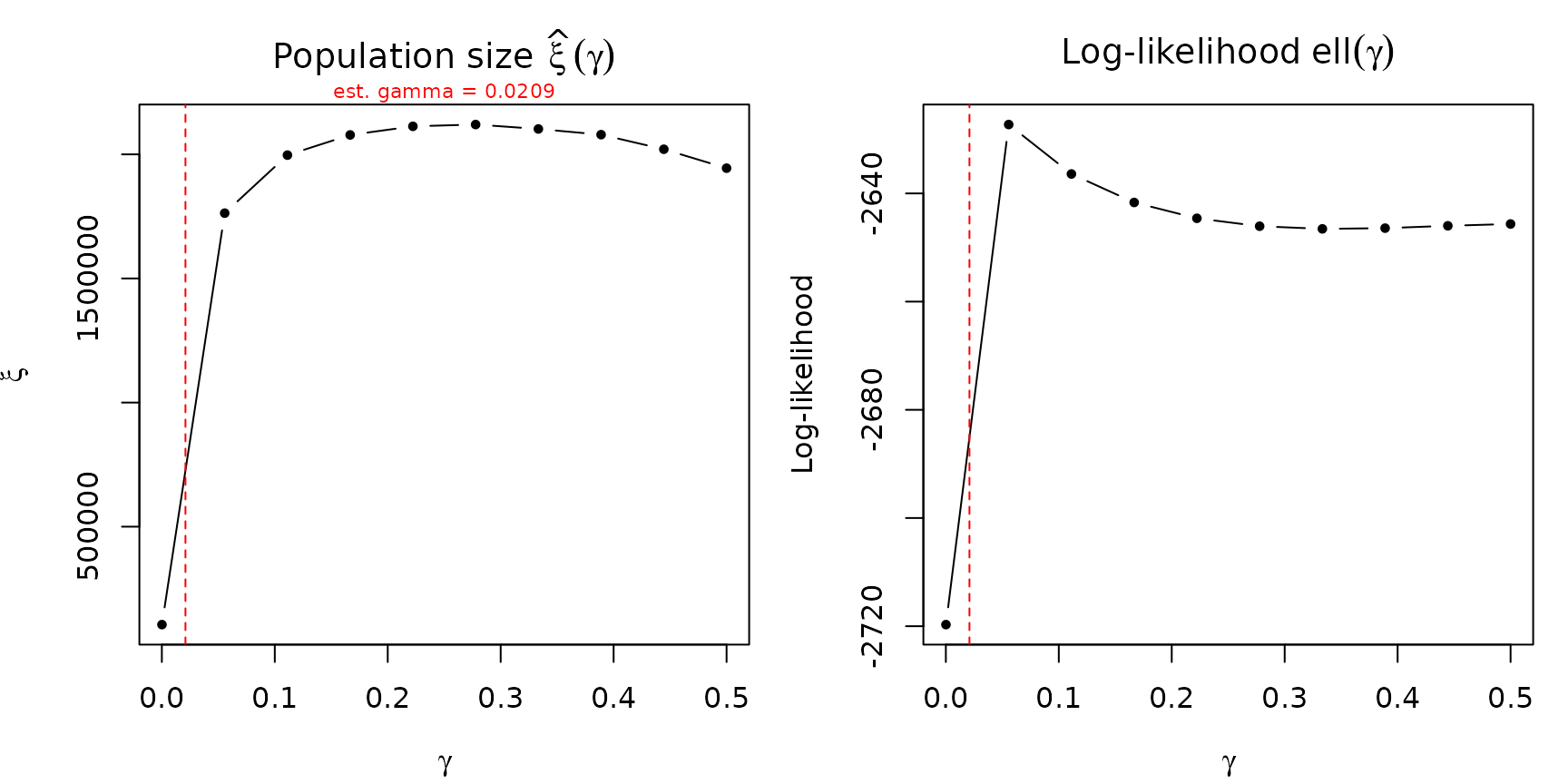

Interpretation:

A sharp peak in the log-likelihood curve means gamma is well-identified by the data. The MLE is precise and the population-size estimate is robust to small perturbations in gamma.
A flat log-likelihood curve means gamma is weakly identified. The data cannot distinguish between a range of gamma values, and the population-size estimate may be sensitive to the gamma assumption. In this case, reporting results for several gamma values (or fixing gamma based on external information) is advisable.

If the original model estimated gamma, its point estimate is marked with a dashed red vertical line. The xi profile shows whether the population-size estimate is stable (flat) or sensitive (steep) across the gamma range.

The profiling results are returned invisibly as a data frame:

prof <- profile_gamma(fit_nb, plot = FALSE)
head(prof)
#>        gamma        xi    loglik
#> 1 0.00010000  105416.4 -2719.707
#> 2 0.02641053 1422974.1 -2621.493
#> 3 0.05272105 1742457.8 -2626.657
#> 4 0.07903158 1892342.5 -2631.701
#> 5 0.10534211 1984163.6 -2635.659
#> 6 0.13165263 2035597.4 -2638.698

References

Beręsewicz, M., & Pawlukiewicz, K. (2020). Estimation of the number of irregular foreigners in Poland using non-linear count regression models. arXiv preprint arXiv:2008.09407.
Kleiber, C. and Zeileis, A. (2016). Visualizing Count Data Regressions Using Rootograms. The American Statistician, 70(3), 296–303.
McCullagh, P. and Nelder, J. A. (1989). Generalized Linear Models, 2nd ed. Chapman & Hall.
Self, S. G. and Liang, K.-Y. (1987). Asymptotic properties of maximum likelihood estimators and likelihood ratio tests under nonstandard conditions. JASA, 82(398), 605–610.
Zhang, L.-C. (2008). Developing methods for determining the number of unauthorized foreigners in Norway (Documents 2008/11). Statistics Norway. https://www.ssb.no/a/english/publikasjoner/pdf/doc_200811_en/doc_200811_en.pdf
Beręsewicz, M., & Pawlukiewicz, K. (2020). Estimation of the number of irregular foreigners in Poland using non-linear count regression models. arXiv preprint arXiv:2008.09407.