Rootogram for count model diagnostics

Compares observed and fitted count frequencies using a rootogram (Kleiber & Zeileis, 2016). Only available for Poisson and Negative Binomial models. Three display styles are supported:

Usage

rootogram(object, ...)

# S3 method for class 'uncounted'
rootogram(
  object,
  style = c("hanging", "standing", "suspended"),
  max_count = NULL,
  sqrt_scale = TRUE,
  ...
)

Arguments

object

An object of class "uncounted" fitted with method = "poisson" or method = "nb".

...

Additional arguments passed to barplot.

style

Character: "hanging" (default), "standing", or "suspended".

max_count

Maximum count value to display. If NULL (default), automatically determined from the data (capped at 100).

sqrt_scale

Logical; use the square-root scale for frequencies (default TRUE).

Value

Invisibly, a list with components observed (observed frequencies), expected (expected frequencies from the fitted model), counts (count values), style, and sqrt_scale.

Details

hanging (default)

Bars representing the observed frequencies are "hung" from the fitted curve. The bottom of each bar should touch the zero line when the fit is good. Deviations below zero indicate underfitting; above zero, overfitting at that count.

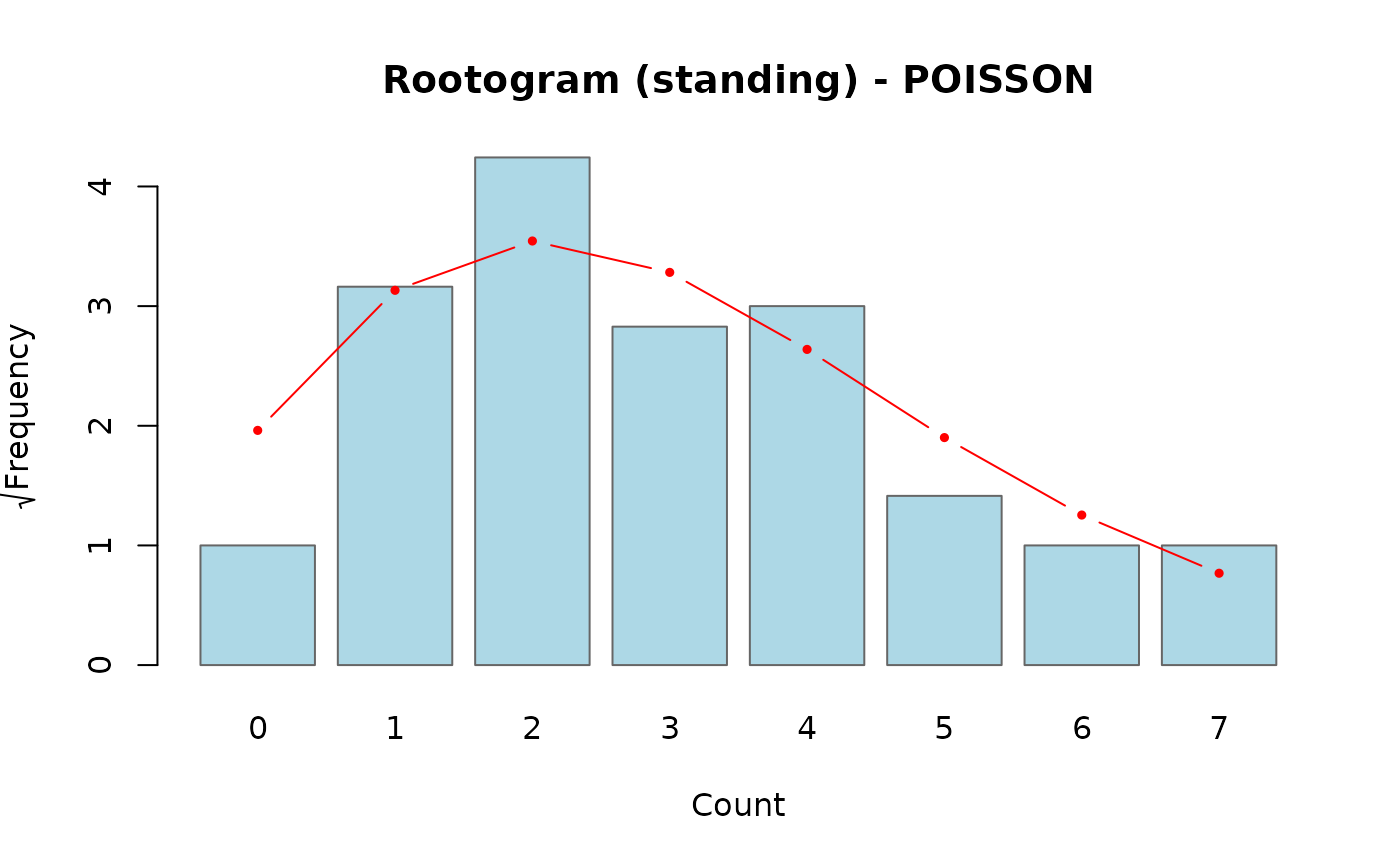
standing

Observed bars stand on the x-axis and the fitted curve is overlaid. Harder to judge discrepancies than the hanging style because the eye must compare bar height to the curve.

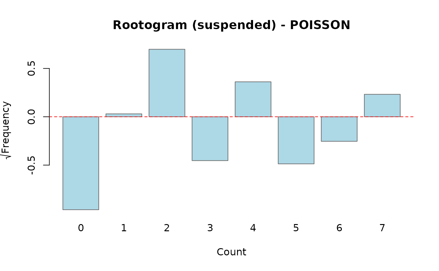
suspended

Plots the difference \(\sqrt{f_{\mathrm{obs}}} - \sqrt{f_{\mathrm{exp}}}\) directly. Bars that cross zero indicate counts where the model over- or under-predicts.

By default the y-axis is on the square-root scale (sqrt_scale = TRUE), which stabilises the visual variability of the bars and makes it easier to judge fit in the tails.

References

Kleiber, C. and Zeileis, A. (2016). Visualizing Count Data Regressions Using Rootograms. The American Statistician, 70(3), 296–303.

Examples

set.seed(123)
df <- data.frame(
  N = rep(1000, 50),
  n = rpois(50, lambda = 50)
)
df$m <- rpois(50, lambda = df$N^0.5 * (df$n / df$N)^0.8)

fit <- estimate_hidden_pop(data = df, observed = ~m, auxiliary = ~n,
                           reference_pop = ~N, method = "poisson")

# Hanging rootogram (default)
rootogram(fit)


# Standing rootogram
rootogram(fit, style = "standing")


# Suspended rootogram
rootogram(fit, style = "suspended")