Compare LOO Results from Two Models — compare

Takes two "uncounted_loo" objects and produces a comparison table and diagnostic plots showing how each observation/country influences the two models differently.

Usage

compare_loo(
  loo1,
  loo2,
  labels = c("Model 1", "Model 2"),
  data = NULL,
  label_vars = NULL
)

Arguments

loo1: An "uncounted_loo" object (first model).
loo2: An "uncounted_loo" object (second model).
labels: Character vector of length 2 with model names. Defaults to c("Model 1", "Model 2").
data: Optional data.table/data.frame with columns matching loo1$dropped identifiers. If provided and LOO is by "obs", columns named label_vars are used to create readable labels.
label_vars: Character vector of column names in data to use for observation labels (e.g., c("country_code", "year", "sex")).

Value

An object of class "uncounted_loo_compare" with components:

table: Data frame sorted by influence, with columns: dropped, label, dxi_<Model1>, pct_<Model1>, dxi_<Model2>, pct_<Model2>, max_abs_pct.
labels: Model labels.
by: The LOO type ("obs" or "country").
dxi_1, dxi_2: Raw $\Delta\xi$ vectors for each model.
pct_1, pct_2: Percentage $\Delta\xi$ vectors.
full_xi_1, full_xi_2: Full-model $\hat{\xi}$ for each model.

Details

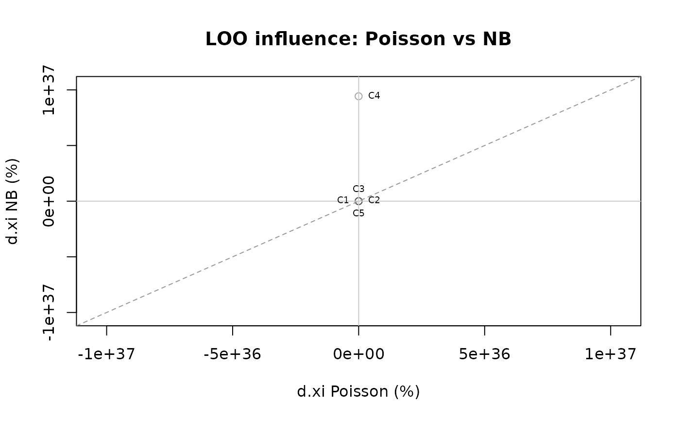
Purpose. When comparing two model specifications (e.g., Poisson vs NB, or different covariate sets), it is useful to check whether the same observations are influential under both models, or whether influence patterns diverge.

Scatter plot interpretation (4 quadrants). The scatter plot (type = "scatter") shows $\%\Delta\xi$ for Model 1 (x-axis) vs Model 2 (y-axis). The four quadrants reveal:

Top-right (+, +): dropping this obs increases $\hat{\xi}$ under both models (obs pulls estimate down in both).
Bottom-left (-, -): dropping this obs decreases $\hat{\xi}$ under both models (obs pulls estimate up in both).
Top-left (-, +): divergent influence – obs pulls the estimate in opposite directions across models.
Bottom-right (+, -): same as top-left but reversed.

Points near the diagonal have similar influence under both models. Points far from the diagonal have divergent influence and warrant investigation.

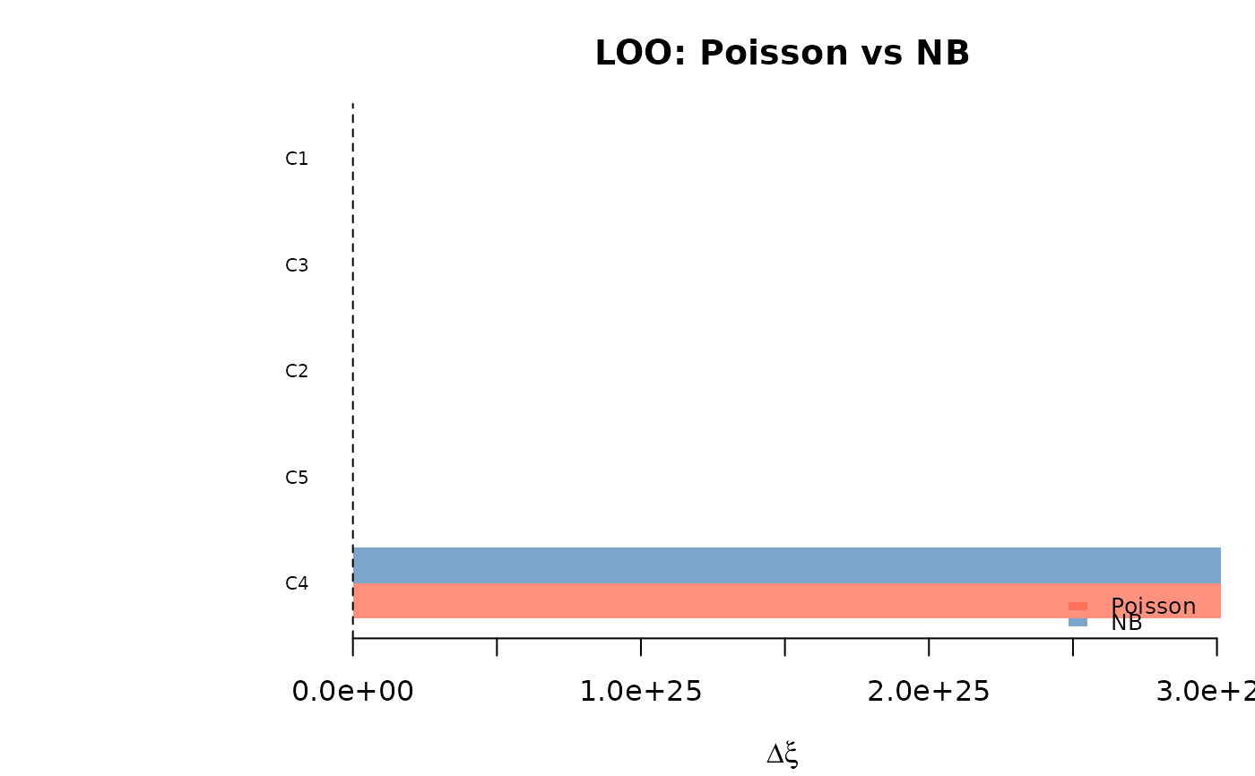
Bar plot. The bar plot (type = "bar") shows the top N most influential observations side by side for both models, ranked by max(|pct_1|, |pct_2|).

Examples

# \donttest{
# Simulate synthetic data
set.seed(42)
n_obs <- 15
sim_data <- data.frame(
  country = rep(paste0("C", 1:5), each = 3),
  year    = rep(2018:2020, 5),
  N       = rpois(n_obs, lambda = 500000),
  n       = rpois(n_obs, lambda = 1000),
  m       = rpois(n_obs, lambda = 50)
)

fit_po <- estimate_hidden_pop(
  data = sim_data, observed = ~m, auxiliary = ~n,
  reference_pop = ~N, method = "poisson",
  countries = ~country
)
#> Warning: Some alpha values < 0 (min = -0.467). Consider using constrained = TRUE.
fit_nb <- estimate_hidden_pop(
  data = sim_data, observed = ~m, auxiliary = ~n,
  reference_pop = ~N, method = "nb",
  countries = ~country
)
#> Warning: Some alpha values < 0 (min = -1.872). Consider using constrained = TRUE.

loo_po <- loo(fit_po, by = "country")
#> Warning: Some alpha values < 0 (min = -3.217). Consider using constrained = TRUE.
#> Warning: Some alpha values < 0 (min = -7.674). Consider using constrained = TRUE.
#> Warning: Some alpha values > 1 (max = 4.281). Population size estimates may be unreliable. Consider using constrained = TRUE or simplifying cov_alpha.
#> Warning: Some alpha values > 1 (max = 2.877). Population size estimates may be unreliable. Consider using constrained = TRUE or simplifying cov_alpha.
loo_nb <- loo(fit_nb, by = "country")
#> Warning: Some alpha values < 0 (min = -3.217). Consider using constrained = TRUE.
#> Warning: Some alpha values < 0 (min = -7.674). Consider using constrained = TRUE.
#> Warning: Some alpha values > 1 (max = 4.281). Population size estimates may be unreliable. Consider using constrained = TRUE or simplifying cov_alpha.
#> Warning: Some alpha values > 1 (max = 2.877). Population size estimates may be unreliable. Consider using constrained = TRUE or simplifying cov_alpha.
comp <- compare_loo(loo_po, loo_nb, labels = c("Poisson", "NB"))
print(comp)
#> LOO comparison: Poisson vs NB 
#> Dropped by: country 
#> Full xi -- Poisson : 0 | NB : 0 
#> 
#> Top 15 most influential (by max |%change|):
#>  label dxi_Poisson   pct_Poisson   dxi_NB       pct_NB        max_abs_pct 
#>  C4     3.012532e+25  9.234739e+28 3.012437e+25  9.425311e+36 9.425311e+36
#>  C5     2.996660e+17  9.186084e+20 2.996660e+17  9.375947e+28 9.375947e+28
#>  C2     3.874090e+03  1.187578e+07 3.874120e+03  1.212134e+15 1.212134e+15
#>  C3    -3.000000e-02 -1.000000e+02 0.000000e+00 -1.000000e+02 1.000000e+02
#>  C1    -3.000000e-02 -1.000000e+02 0.000000e+00 -1.000000e+02 1.000000e+02
plot(comp, type = "scatter")

plot(comp, type = "bar")

# }