Introduction
This vignette demonstrates how to compare estimation methods and present results using the uncounted package’s plotting and reporting tools.
Fitting multiple models
The package supports five estimation methods. We fit Poisson, NB, and iOLS to the same data for comparison:
fit_po <- estimate_hidden_pop(d, ~ m, ~ n, ~ N,
  method = "poisson", cov_alpha = ~ year + sex,
  gamma = "estimate", countries = ~ country_code)

fit_nb <- estimate_hidden_pop(d, ~ m, ~ n, ~ N,
  method = "nb", cov_alpha = ~ year + sex,
  gamma = fit_po$gamma, countries = ~ country_code)

fit_io <- estimate_hidden_pop(d, ~ m, ~ n, ~ N,
  method = "iols", cov_alpha = ~ year + sex,
  gamma = fit_po$gamma, countries = ~ country_code)
Coefficient tables with modelsummary
The package provides tidy() and glance()
methods compatible with the modelsummary package:
library(modelsummary)
modelsummary(
  list(Poisson = fit_po, NB = fit_nb, iOLS = fit_io),
  stars = TRUE
)| Poisson | NB | iOLS | |
|---|---|---|---|
| + p < 0.1, * p < 0.05, ** p < 0.01, *** p < 0.001 | |||
| alpha × (Intercept) | 0.772*** | 0.867*** | 0.764*** |
| (0.050) | (0.026) | (0.065) | |
| alpha × year2020 | -0.062** | -0.112*** | -0.116*** |
| (0.022) | (0.016) | (0.024) | |
| alpha × year2021 | -0.093*** | -0.148*** | -0.169*** |
| (0.023) | (0.019) | (0.026) | |
| alpha × year2022 | -0.122*** | -0.127*** | -0.141*** |
| (0.025) | (0.018) | (0.028) | |
| alpha × year2023 | -0.097* | -0.077*** | -0.092*** |
| (0.046) | (0.016) | (0.021) | |
| alpha × year2024 | -0.060 | 0.008 | -0.008 |
| (0.058) | (0.016) | (0.020) | |
| alpha × sexMale | 0.042 | 0.017 | 0.049* |
| (0.038) | (0.012) | (0.023) | |
| beta | 0.613*** | 0.783*** | 0.638*** |
| (0.122) | (0.032) | (0.071) | |
| gamma | 0.006 | ||
| (0.005) | |||
| theta | 1.276 | ||
| (0.084) | |||
| Num.Obs. | 1382 | 1382 | 1382 |
| AIC | 17569.0 | 5303.9 | 925616.0 |
| BIC | 17616.1 | 5351.0 | 925657.9 |
| Log.Lik. | -8775.519 | -2642.969 | -462800.005 |
| method | POISSON | NB | IOLS |
Individual coefficient tables:
tidy(fit_po, conf.int = TRUE)
#>                term    estimate   std.error statistic      p.value     conf.low
#> 1 alpha:(Intercept)  0.77178227 0.050387227 15.317022 5.885272e-53  0.673025123
#> 2    alpha:year2020 -0.06192409 0.021868389 -2.831671 4.630544e-03 -0.104785341
#> 3    alpha:year2021 -0.09301571 0.022994523 -4.045124 5.229535e-05 -0.138084143
#> 4    alpha:year2022 -0.12230318 0.024719168 -4.947706 7.509323e-07 -0.170751855
#> 5    alpha:year2023 -0.09657813 0.045874342 -2.105276 3.526732e-02 -0.186490193
#> 6    alpha:year2024 -0.05981457 0.057933917 -1.032462 3.018557e-01 -0.173362962
#> 7     alpha:sexMale  0.04179194 0.037663367  1.109618 2.671638e-01 -0.032026900
#> 8              beta  0.61326713 0.122280967  5.015230 5.297016e-07  0.373600839
#> 9             gamma  0.00608425 0.005101258        NA           NA  0.001176328
#>      conf.high
#> 1  0.870539424
#> 2 -0.019062831
#> 3 -0.047947269
#> 4 -0.073854496
#> 5 -0.006666075
#> 6  0.053733821
#> 7  0.115610785
#> 8  0.852933422
#> 9  0.031469196
glance(fit_po)
#>    method nobs    logLik      AIC      BIC deviance df.residual
#> 1 POISSON 1382 -8775.519 17569.04 17616.12 14948.24        1373
Plotting population size estimates
The popsize() function returns an object that can be
plotted directly:

# Compare plug-in vs bias-corrected
plot(ps, type = "compare")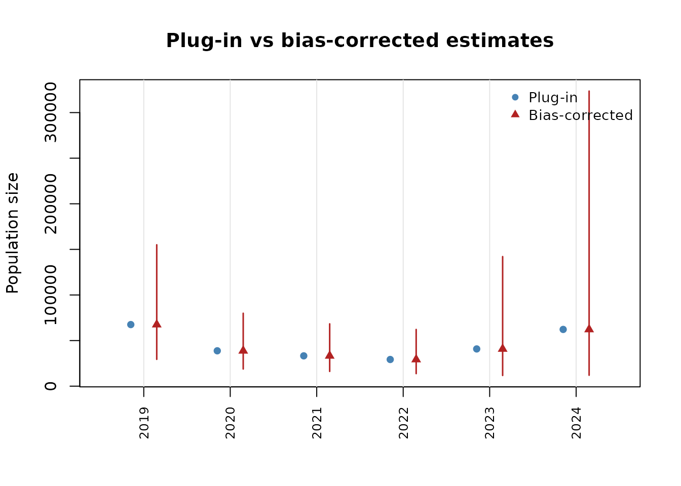
Comparing models visually
compare_popsize() produces side-by-side population size
estimates:
comp <- compare_popsize(fit_po, fit_nb, fit_io,
  labels = c("Poisson", "NB", "iOLS"),
  by = ~ year)

print(comp)
#> Population size comparison: Poisson vs NB vs iOLS
#>
#>      model group  estimate estimate_bc      lower     upper
#> 1  Poisson  2019  67536.84    67504.29  29387.550 155059.84
#> 2  Poisson  2020  38787.40    38766.50  18790.590  79978.43
#> 3  Poisson  2021  33243.01    33224.95  16150.801  68349.37
#> 4  Poisson  2022  29249.61    29233.11  13739.451  62198.63
#> 5  Poisson  2023  40825.92    40804.83  11715.868 142117.88
#> 6  Poisson  2024  62218.64    62188.79  11951.536 323594.02
#> 7       NB  2019 156232.49   152016.66  94807.822 243746.39
#> 8       NB  2020  51814.02    50505.32  33151.839  76942.56
#> 9       NB  2021  42132.35    41172.74  25999.219  65201.73
#> 10      NB  2022  63811.40    62276.29  39962.929  97048.35
#> 11      NB  2023 116535.58   113818.33  71444.483 181324.17
#> 12      NB  2024 305601.66   298353.19 182612.635 487450.53
#> 13    iOLS  2019  65745.65    64612.51  22417.088 186231.87
#> 14    iOLS  2020  21998.78    21671.81   8247.433  56947.12
#> 15    iOLS  2021  15444.44    15246.53   5642.191  41199.73
#> 16    iOLS  2022  23655.49    23334.48   8887.972  61262.34
#> 17    iOLS  2023  41622.40    41061.39  15118.868 111518.80
#> 18    iOLS  2024 104625.35   103172.19  37066.217 287175.24
plot(comp)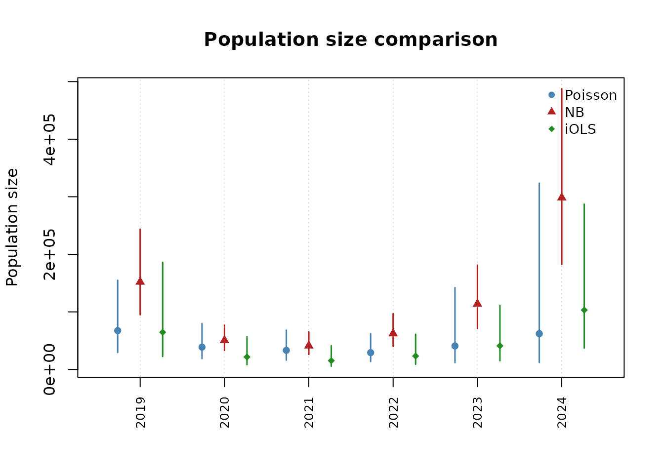
Predictions
The predict() method supports new data:
# Fitted values
head(predict(fit_po))
#> [1]  3.2837249  0.3538453  2.3653566  2.2142433 21.0701264  0.8119227

# Log-scale (linear predictor)
head(predict(fit_po, type = "link"))
#> [1]  1.1889784 -1.0388955  0.8609288  0.7949107  3.0478562 -0.2083502

# Predictions for new data
new_d <- d[1:10, ]
predict(fit_po, newdata = new_d)
#>  [1]  3.2837249  0.3538453  2.3653566  2.2142433 21.0701264  0.8119227
#>  [7]  3.9496912  2.1480204  0.4921352 84.9170469
Model selection guidance
| Situation | Recommended method |
|---|---|
| Default analysis | Poisson (robust, well-studied) |
| Overdispersion suspected | NB, then LR test vs Poisson |
| Sensitivity to large countries | iOLS alongside Poisson |
| Quick exploration | OLS with fixed gamma |
When Poisson and iOLS agree, the result is robust to the choice of weighting. When they diverge, report both and discuss which observations drive the difference.
References
- Santos Silva, J. M. C. & Tenreyro, S. (2006). The Log of Gravity. Review of Economics and Statistics, 88(4), 641–658.
- Benatia, D., Bellego, C. & Pape, L.-D. (2024). Dealing with Logs and Zeros in Regression Models. arXiv:2203.11820v3.
- Zhang, L.-C. (2008). Developing methods for determining the number of unauthorized foreigners in Norway (Documents 2008/11). Statistics Norway.
- Beresewicz, M. & Pawlukiewicz, K. (2020). Estimation of the number of irregular foreigners in Poland using non-linear count regression models. arXiv:2008.09407.