nonprobsvy -- An R Package for Modern Methods for Non-Probability Surveys

Łukasz Chrostowski (Analytic Partners)

Piotr Chlebicki (Stockholm University)

Maciej Beręsewicz (Poznań University of Economics and Business; Statistical Office in Poznań)

2026-05-22

Abstract. The paper presents nonprobsvy – an R package for inference based on non-probability samples. The package implements various approaches that can be categorized into three groups: prediction-based approach, inverse probability weighting and doubly robust approach. In the package, we assume the existence of either population-level data or probability-based population information and leverage the survey package for inference. The package implements both analytical and bootstrap variance estimation for the proposed estimators. In the paper we present the theory behind the package, its functionalities and a case study that showcases the usage of the package. The package is aimed at scientists and researchers who would like to use non-probability samples (e.g., big data, opt-in web panels, social media) to accurately estimate population characteristics.

Keywords: data integration, doubly robust estimation, propensity score estimation, mass imputation, survey.

Introduction

In official statistics, information about the target population and its characteristics is mainly collected through probability surveys, censuses or is obtained from administrative registers and covers all (or nearly all) units of the population. However, owing to increasing non-response rates, particularly unit non-response and non-contact, which result from the growing respondent burden as well as rising costs of surveys conducted by National Statistical Institutes, non-probability data sources are becoming more popular (Beręsewicz 2017; Beaumont 2020; Biffignandi and Bethlehem 2021). Non-probability surveys, such as opt-in web panels, social media, scanner data, mobile phone data or voluntary register data, are currently being explored for use in the production of official statistics (Citro 2014; Daas et al. 2015), public opinion studies (Schonlau and Couper 2017) or market research (cf. Grow et al. 2022). Since the selection mechanism underlying these sources is unknown, standard design-based inference methods cannot be directly applied and, in the case of large datasets, can lead to the big data paradox, i.e., the larger the sample, the larger the bias, as described by Meng (2018).

Table 1 compares basic characteristics of probability and non-probability samples. In particular, it shows the advantages and disadvantages of each type with respect to the selection mechanism, the population coverage, bias, variance, costs and timeliness. In general, the quality of non-probability samples suffers from an unknown selection mechanism (i.e., unknown probabilities of inclusion) and under-coverage of certain groups from the population (e.g., older people). As a result, direct estimates based on non-probability samples are biased and, in most cases, are characterized by small variance owing to their size. Certainly, the costs and timeliness of these surveys are significantly smaller than those of probability samples.

Table 1. A comparison of probability and non-probability samples and their characteristics.

Factor	Probability sample	Non-probability sample
Selection	Known probabilities	Unknown probabilities (self-selection)
Coverage	Complete	May be incomplete
Estimation bias	Unbiased under design	Potential systematic bias
Variance of estimates	Typically high	Typically low
Cost	High	Low
Timeliness	Long delay	Very short delay

To address this problem, several approaches have been proposed, which rely on the estimation of propensity scores (PS; i.e., inclusion probabilities) for deriving inverse probability weights (IPW; also known as propensity score weighting/adjustment, cf. Lee (2006; Lee and Valliant 2009)), on model-based prediction (in particular, mass imputation estimators; MI) and on the doubly robust (DR) approach involving IPW and MI estimators. Two main scenarios are usually considered:

1. only population-level means or totals are available (e.g., from census, registers or sample surveys),
2. unit-level data are available either in the form of registers covering the whole population or in the form of probability surveys (cf. Elliott and Valliant 2017).

Wu (2022) classified these approaches into three groups that require a joint randomization framework involving a probability sampling design (denoted as p) and an outcome regression model (denoted as \xi) or a PS model (denoted as q). According to this classification, IPW estimators represent the qp framework, MI estimators represent the \xi p framework, and DR estimators can represent either the qp or the \xi p framework.

Most approaches assume that population data is available in order to reduce the bias of non-probability sampling by reweighting to reproduce known population totals/means (i.e., IPW estimators); by modeling the target variable using various techniques (i.e., MI estimators); or by combining both approaches (e.g., DR estimators, cf. Chen et al. (2020); see also multilevel regression and post-stratification, MRP; Mister-P, cf. Gelman (1997)). This topic has become very popular and a number of new methods have been proposed; for instance non-parametric approaches based on nearest neighbors (Yang et al. 2021), kernel density estimation (Chen et al. 2022), empirical likelihood (Kim and Morikawa 2023), model-calibration with LASSO (Chen et al. 2018) or quantile balanced IPW (Beręsewicz et al. 2025) to name a few. It should be highlighted that, in contrast to probability samples, there is no single method that can be used for all non-probability samples. Based on the methods available in the literature several statistical software solutions have been developed. These pieces of software will be presented and compared with nonprobsvy (Chrostowski et al. 2025) in the next section.

Software for non-probability samples

Table 2 presents a comparison of selected packages in terms of the availability of different inference methods. The reason for this is the availability of software designed for inference based on non-probability samples, not a general way to estimate propensity scores or model \mathbb{E}(Y \mid X). For such reviews, one can refer to Valliant and Dever (2018, chap. 6) who discussed weighting and matching in this context in Stata (StataCorp 2025) using logit, svy and teffects nnmatch commands or Lohr (2021, e.g., Chapter 8) who covers SAS software [ Institute Inc. (2023); e.g., PROC LOGISTIC procedure].

We focus on packages available as open source or via CRAN or PyPI (for non-CRAN or non-PyPI software see Cobo et al. (2024)). Our comparison includes five packages that focus specifically on non-probability sampling: in R – NonProbEst (Mart’ın et al. 2020) and our nonprobsvy, and in Python – balance (Sarig et al. 2023), inps (Castro 2024), and in Stan (Carpenter et al. 2017) e.g., through the R package rstanarm, which allows you to easily apply the rstanarm’s MRP method (Goodrich et al. 2024).

Table 2. A comparison of packages and implemented methods.

	Stan	balance (Python)	inps (Python)	NonProbEst (R)	nonprobsvy (R)
IPW	–	✓	✓	✓	✓
Calibrated IPW	–	–	–	–	✓
MI	–	–	–	✓	✓
DR	–	–	✓	–	✓
MRP	✓	–	–	–	–
Variable selection	✓	✓	✓	✓	✓
Analytical variance	–	–	–	–	✓
Bootstrap variance	–	–	–	✓	✓
Integration with survey/samplics	–	–	–	–	✓

The NonProbEst package, while more limited than nonprobsvy, offers various techniques, such as PS or prediction approaches (e.g., model-calibrated). Users can choose several different settings for PS weights, variable selection and can estimate variance of the mean using the leave-one-out Jackknife procedure. Unfortunately, the package is no longer actively developed (as of August 2025) and some of the techniques are either outdated or have been shown to be inappropriate for non-probability samples. While the package contains functions designed for specific methods, it does not allow users to leverage the survey package (Lumley 2004) for estimation. The balance package is solely dedicated to the PS approach (as of version 0.10.0). It assumes that the reference probability sample is available and the authors have implemented the variance estimator of the weighted mean as a measure of uncertainty for the IPW estimator. The weights for the IPW estimator are constructed using the approach proposed by Schonlau and Couper (2017). The inps package supports the use of unit-level data from a probability sample or the population, implements IPW, MI and DR estimators, and offers users the possibility of selecting variables but is still at a very early stage of development. It also implements kernel weighting and a simple bootstrap approach via the scipy.stats package (Virtanen et al. 2020). Neither balance nor inps supports the use of the samplics package (Diallo 2021). Finally, we note that the MRP approach is implemented solely in Stan with variable selection specified by an appropriate prior, but it can be easily implemented in other probabilistic programming languages, e.g., using the Turing.jl package (Fjelde et al. 2025) in the Julia language (Bezanson et al. 2017).

The nonprobsvy package has several advantages over those presented above. Firstly, it implements state-of-the-art methods recently proposed in the literature, along with valid statistical inference procedures. Secondly, it offers other approaches, such as calibrated IPW (where PS weights match either the population or estimated totals), NN and PMM matching, various IPW and DR estimators using generalized linear models (GLM) with different link functions for probability estimation. Thirdly, it supports the functions included in the survey package to account for the design of the probability sample. Finally, we provide a user-friendly API that mimics glm(), survey::calibrate() and other functions known in R, together with the main function to specify the approach and estimators. As far as we know, the nonprobsvy is the only software (open-access or commercial) that offers such functionalities.

The remaining part of the paper is structured as follows. The next section is dedicated to the theory of statistical inference based on non-probability samples. We provide the basic set-up and introduce specific methods in separate sections. We follow the notation used by Wu (2022) throughout the paper. We then describe the main function and the package functionalities, and present an empirical study showcasing the process of integrating data from the Polish Job Vacancy Survey with voluntary administrative data from the Central Job Offers Database in order to estimate the number of companies with at least one vacancy offered on a single shift. We then present classes and S3 methods implemented in the package. The paper ends with a summary and plans for future development. The Appendix presents algorithms for selected MI estimators.

The package nonprobsvy (Chrostowski et al. 2025) is available from the Comprehensive R Archive Network (CRAN) at https://CRAN.R-project.org/package=nonprobsvy.

Methods for non-probability samples

Basic setup

Let U = \{1, \ldots, N\} denote the target population consisting of N labeled units. Each unit i has an associated L-dimensional vector of auxiliary variables \boldsymbol{x}_{i} and the study (target) variable y_{i}. Let \{ (y_i, \boldsymbol{x}_i), i \in \mathcal{I}_{\text{NP}}\} be a non-probability sample S_{\text{NP}} of size n_{\text{NP}}, where \mathcal{I}_{\text{NP}} is an index set for S_{\text{NP}}. Let \left\{\left(\boldsymbol{x}_i, \pi_{\text{P},i}\right), i \in \mathcal{I}_{\text{P}}\right\} be a probability sample S_{\text{P}} of size n_{\text{P}}, where \mathcal{I}_{\text{P}} is an index set for S_{\text{P}}, and the only information known for all units in the population refers to auxiliary variables \boldsymbol{x} and inclusion probabilities \pi_{\text{P}}. Each unit in the S_{\text{P}} sample has been assigned a design-based weight given by d_{\text{P},i} = 1/\pi_{\text{P},i}.

Let I_{\text{NP},i}=I(i \in S_{\text{NP}}) and I_{\text{P},i}=I(i \in S_{\text{P}}) be indicators of inclusion in the non-probability sample S_{\text{NP}} and the probability sample S_{\text{P}}, respectively, which are defined for all units in the target population. Let \pi_{\text{NP},i}=\mathbb{P}(I_{\text{NP},i}=1 \mid \boldsymbol{x}_i, y_i)=\mathbb{P}(I_{\text{NP},i}=1 \mid \boldsymbol{x}_i) be propensity scores, which characterize the S_{\text{NP}} sample’s inclusion and participation mechanisms. Unlike \pi_{\text{P},i}, the \pi_{\text{NP},i} and d_{\text{NP},i}=1/\pi_{\text{NP},i} are unknown. The description of the data is presented in a more concise form in Table 3.

Table 3. Two-sample setting with no overlap between samples.

Sample	ID	Inclusion (I_{\text{NP}})	Design weight (d)	Covariates (\boldsymbol{x})	Study variable (y)
Non-probability	1	1	?	✓	✓
S_{\text{NP}}	⋮	⋮	⋮	⋮	⋮
	n_{\text{NP}}	1	?	✓	✓
Probability	n_{\text{NP}}+1	0	✓	✓	?
S_{\text{P}}	⋮	⋮	⋮	⋮	⋮
	n_{\text{NP}}+n_{\text{P}}	0	✓	✓	?

The goal is to estimate the finite population mean \mu_{y} = N^{-1}\sum_{i=1}^{N} y_{i} of the target variable y. As values of y_{i} are not observed in the probability sample, they cannot be used to estimate the target quantity. Instead, one could try combining the non-probability and probability samples (or known population totals) to estimate \mu_{y}. Given the absence of a universally accepted method for achieving this objective, assumptions vary considerably, as outlined by Wu (2022). However, the following are the main assumptions that apply to the majority of methods presented in this section:

• A1 I_{\text{NP}, i} and the study variable y_{i} are independent given the set of covariates \boldsymbol{x}_{i} (the missing at random mechanism).
• A2 All the units in the target population have non-zero PS, i.e., \pi_{\text{NP}, i}>0, i=1, 2, \ldots, N (i.e., no coverage error).
• A3 The indicator variables I_{\text{NP}, 1}, I_{\text{NP}, 2}, \ldots, I_{\text{NP}, N} are independent given the set of auxiliary variables \left(\boldsymbol{x}_1, \boldsymbol{x}_2, \ldots, \boldsymbol{x}_N\right) (i.e., no clustering).

Currently, we ignore overlap between S_{\text{NP}} and S_{\text{P}}, and assume no measurement error in y_i and the fact that values of \boldsymbol{x}_i are known. The setting presented in Table 3 can also be extended to calibrated d_{\text{P}, i} weights (i.e., d_{\text{P}, i} adjusted for under-coverage, non-contact or non-response; cf. Särndal and Lundström (2005)) but this requires additional developments in the theory about the consistency of the MI, IPW and DR estimators. In the next sections we briefly present the methods implemented in the package.

Prediction-based approach

Prediction estimators

In the prediction approach the following semi-parametric model for the finite population is assumed:

\mathbb{E}_{\xi}\left(y_i \mid \boldsymbol{x}_i\right)=m\left(\boldsymbol{x}_i, \boldsymbol{\beta}\right), \text { and } \quad V_{\xi}\left(y_i \mid \boldsymbol{x}_i\right)=v\left(\boldsymbol{x}_i\right) \sigma^2, \quad i=1, 2, \ldots, N, \tag{1}

where the mean function m(\cdot, \cdot) and the variance v(\cdot) have known forms, \boldsymbol{\beta} and \sigma^2 are model parameters and y_i are also assumed to be conditionally independent given the \boldsymbol{x}_i. The model in Equation 1 is assumed to hold for all units in the non-probability sample S_{\text{NP}}. The parameters of the model in Equation 1 can be estimated using the quasi maximum likelihood estimation method, which includes linear and non-linear models, such as GLM. Let \boldsymbol{\beta}_0 and \sigma^2_0 be the true values of the model parameters \boldsymbol{\beta} and \sigma^2 under the adopted model and \hat{\boldsymbol{\beta}} be the quasi maximum likelihood estimator of \boldsymbol{\beta}_0. Let m_i=m(\boldsymbol{x}_i, \boldsymbol{\beta}_0) and \hat{m}_i=m(\boldsymbol{x}_i, \hat{\boldsymbol{\beta}}) be calculated for all units i=1, \ldots, N. Under this setting, as Wu (2022) notes, there are two commonly used prediction estimators:

\hat{\mu}_{y, \text{PR1}}=\frac{1}{N} \sum_{i=1}^N \hat{m}_i \quad \text { and } \quad \hat{\mu}_{y, \text{PR2}}=\frac{1}{N}\left\{\sum_{i \in S_{\text{NP}}} y_i-\sum_{i \in S_{\text{NP}}} \hat{m}_i+\sum_{i=1}^N \hat{m}_i\right\}. \tag{2}

Under linear models, where m(\boldsymbol{x}_i, \boldsymbol{\beta})=\boldsymbol{x}_i^{\top}\boldsymbol{\beta}, the two estimators in Equation 2 reduce to:

\hat{\mu}_{y, \text{PR1}}=\mu_{\boldsymbol{x}}^{\top} \hat{\boldsymbol{\beta}} \quad \text { and } \quad \hat{\mu}_{y, \text{PR2}}=\frac{n_{\text{NP}}}{N}\left(\overline{y}_{\text{NP}}-\overline{\boldsymbol{x}}_{\text{NP}}^{\top} \hat{\boldsymbol{\beta}}\right)+\mu_{\boldsymbol{x}}^{\top} \hat{\boldsymbol{\beta}}, \tag{3}

where \mu_{\boldsymbol{x}} = N^{-1}\sum_{i=1}^N\boldsymbol{x}_i is the vector of the population means of the \boldsymbol{x} variables and \overline{\boldsymbol{x}}_{\text{NP}}=n_{\text{NP}}^{-1}\sum_{i \in S_{\text{NP}}}\boldsymbol{x}_i is the vector of the simple means of \boldsymbol{x} from the non-probability S_{\text{NP}} sample. If the linear model contains an intercept and \hat{\boldsymbol{\beta}} is the ordinary least squares estimator, then \hat{\mu}_{y, \text{PR1}}=\hat{\mu}_{y, \text{PR2}}.

The estimator in Equation 3 is appealing as it only requires the non-probability sample S_{\text{NP}} and reference population means (or totals and population size N). If the population means are unknown, they can be replaced by estimates provided by the reference probability sample S_{\text{P}}, i.e., \sum_{i=1}^N \hat{m}_i is replaced with \sum_{i \in S_{\text{P}}} d_{\text{P}, i}\hat{m}_i for Equation 2 and \mu_{\boldsymbol{x}} is replaced by \hat{\mu}_{\boldsymbol{x}}=\hat{N}_{\text{P}}^{-1}\sum_{i \in S_{\text{P}}}d_{\text{P}, i}\boldsymbol{x}_i for Equation 3 where \hat{N}_{\text{P}}=\sum_{i \in S_{\text{P}}}d_{\text{P}, i}.

Mass imputation estimators

Model-based prediction estimators of \mu can be treated as mass imputation estimators, since the information on y_i is missing entirely in the reference probability sample S_{\text{P}} (but \boldsymbol{x}_i is available) and y_i can be imputed based on the non-probability sample as values of \{ (y_i, \boldsymbol{x}_i), i \in \mathcal{I}_{\text{NP}}\} are known. The general form of the MI estimator is given by:

\hat{\mu}_{y, \text{MI}}=\frac{1}{\hat{N}_{\text{P}}} \sum_{i \in S_{\text{P}}} d_{\text{P}, i} y_i^*,

where y_i^* is the imputed value of y_i and \hat{N}_{\text{P}} is defined as previously. Under deterministic regression imputation, the \hat{\mu}_{y, \text{MI}} estimator reduces to the estimators in Equation 2.

There are several ways of imputing y_i^* and in the nonprobsvy package we have implemented the following MI estimators: the semi-parametric approach based on GLM (MI-GLM), kernel smoothing (MI-NPAR), nearest neighbor matching (MI-NN) and predictive mean matching (MI-PMM).

The properties of the MI-GLM estimator, where y_i^* are imputed with \hat{m}_i from the semi-parametric model, were studied by Kim et al. (2021). In the nonprobsvy package, we account for the following GLM families: gaussian(), binomial() and poisson(). The MI-NPAR estimator was proposed by Chen et al. (2022) who studied its finite population properties. Currently, we implement this approach using local polynomial regression using stats::loess() function. In the next releases we will allow users to use the np (Hayfield and Racine 2008) or KernSmooth (Wand 2025) packages.

The MI-NN estimator was initially proposed by Rivers (2007) under the name sample matching and theoretical properties of the MI-NN estimator for large non-probability samples (big data, i.e., covering a significant part of the target population) were studied by Yang et al. (2021). The basic idea of NN matching is as follows:

1. for each unit i in the probability sample S_{\text{P}} find a donor j (or multiple donors) in the S_{\text{NP}} sample based on some distance between \boldsymbol{x}_i and \boldsymbol{x}_j,
2. use the matched values y_j from S_{\text{NP}} to impute missing y_i values in the probability sample S_{\text{P}}.

Imputed values of y_i^* depend on the number of selected k neighbors: for k=1, the closest unit is selected, and for k>1, one can calculate a simple average over a vector of selected y values. A detailed description of the procedure is presented in Algorithm 1 in the Appendix. The MI-NN estimator suffers from the curse of dimensionality, i.e., asymptotic bias of the MI estimator increases as the number of covariates \boldsymbol{x} increases with a fixed k (Abadie and Imbens 2006; Yang and Kim 2020). The single PMM imputation approach has been proposed to overcome this issue (Chlebicki et al. 2024).

In the PMM approach, matching is done using predicted values of \hat{m}_i=m\left(\boldsymbol{x}_i, \hat{\boldsymbol{\beta}}\right) instead of \boldsymbol{x}_i, thus the NN algorithm is modified as follows:

1. fit the model m\left(\boldsymbol{x}_i, \boldsymbol{\beta}\right) to non-probability S_{\text{NP}} sample,
2. assign predicted values \hat{m}_i to all units in S_{\text{NP}} and S_{\text{P}},
3. match all units from the S_{\text{P}} sample to donor units from the S_{\text{NP}} sample based on \hat{m} values.

The MI-PMM estimator is the same as in the NN approach but differs from the multiple imputation PMM implemented in the mice package (van Buuren and Groothuis-Oudshoorn 2011). In nonprobsvy we have implemented a single imputation method (i.e., one dataset is created). Chlebicki et al. (2024) studied properties of two variants of the MI-PMM estimator for non-probability samples: matching predicted to predicted (\hat{m}-\hat{m} matching; denoted as MI-PMM-A) and matching predicted to observed (\hat{m}-y matching; denoted as MI-PMM-B). Details of the procedure can be found in Algorithm 2 and Algorithm 3 in the Appendix. Chlebicki et al. (2024) also prove the consistency of the MI-PMM-A estimator under model misspecification, i.e., the assumed model may differ from the true one.

Variance estimators for the prediction approach

Variance of the MI estimators can be estimated analytically or using the bootstrap approach. The analytical estimator of the variance of the MI-GLM estimator proposed by Kim et al. (2021, 950) contains two components: \hat{V}_1 (based on the information from both samples S_{\text{NP}} and S_{\text{P}}) and \hat{V}_2 (based exclusively on the probability sample S_{\text{P}}). For the MI-NN estimator Yang et al. (2021) proposed a variance estimator for large S_{\text{NP}} samples, which reduces to the part for the probability sample S_{\text{P}} (i.e., the design-based variance estimator of the mean, which can easily be obtained from the survey package) and a version for smaller samples can be found in Chlebicki et al. (2024). With respect to the variance of MI-PMM estimators, Chlebicki et al. (2024) propose formulas which are the same as those for the MI-NN estimators. The analytical variance estimator for the MI-NPAR was proposed by Chen et al. (2022).

In the bootstrap approach each bootstrap replication b=1, \ldots, B consists of the following steps.

1. Independently:
   • Draw a simple random sampling with replacement from the non-probability sample S_{\text{NP}} (using base::sample() function).
   • Draw a sample according to the declared sampling design from the probability sample S_{\text{P}} (e.g., one can use the as.svrepdesign() function from the survey package).
2. Estimate \mu_{y, \text{MI}}^b using an appropriate approach (e.g., MI-GLM, MI-NN or MI-PMM).

After obtaining B bootstrap replicates, estimate variance using the following equation:

\hat{V}_{\text{boot}} = \frac{1}{B-1}\sum_{b=1}^B\left(\hat{\mu}^b_{y, \text{MI}} - \hat{\mu}_{y, \text{MI}}\right)^2. \tag{4}

The above approaches are applied when unit-level data from the probability sample S_{\text{P}} are available. If this is not the case and only population means (or totals and population size) are available, we can estimate the variance of the \mu_{y, \text{MI-GLM}} estimator using the first component \hat{V}_1 of the Kim et al. (2021) variance estimator (replaced by the survey-based population quantities, if available). To estimate the variance of the MI-NN and MI-PMM estimators we only allow the bootstrap approach with known population means. Note that the current version of the nonprobsvy does not support the use of replicated weights in the probability sample S_{\text{P}} for any of the estimators discussed in this paper.

Inverse probability weighting

Inverse probability weighting, another popular estimation approach, involves estimating PS given by \pi_{\text{NP}, i}=\mathbb{P}\left(i \in S_{\text{NP}} \right). As in the case of the prediction-based approach, there are two variants of the IPW estimator, given by:

\hat{\mu}_{y, \text{IPW-HT}}=\frac{1}{N} \sum_{i \in S_{\text{NP}}} \frac{y_i}{\hat{\pi}_{\text{NP}, i}} \quad \text{and} \quad \hat{\mu}_{y, \text{IPW-Hájek}}=\frac{1}{\hat{N}_{\text{NP}}} \sum_{i \in S_{\text{NP}}} \frac{y_i}{\hat{\pi}_{\text{NP}, i}}, \tag{5}

where the \hat{\mu}_{y, \text{IPW-HT}} is an adjustment of the Horvitz-Thompson estimator, and the \hat{\mu}_{y, \text{IPW-Hájek}} is an adjustment of the Hájek estimator, where the estimated population size is given by \hat{N}_{\text{NP}} = \sum_{i \in S_{\text{NP}}} \hat{\pi}_{\text{NP}, i}^{-1}. The use of this estimator with respect to non-probability samples is discussed by Lee (2006) and Biffignandi and Bethlehem (2021, chap. 13) and there are several approaches to using propensity scores along with alternative versions of the weights (cf. Elliott and Valliant 2017, sec. 3). In an article by Chen et al. (2020) dedicated to the properties of the estimators in Equation 5, the authors proved their consistency and derived their closed form versions. Wu (2022, sec. 4.2) argues that the \hat{\mu}_{y, \text{IPW-Hájek}} estimator performs better than \hat{\mu}_{y, \text{IPW-HT}} even if the population size is known.

The construction of the IPW estimator involves two steps:

1. estimating the PS,
2. deriving d_{\text{NP}, i} weights (which, in our case, are equal to \pi_{\text{NP}, i}^{-1})

To estimate the propensity scores \pi_{\text{NP}, i}=\pi(\boldsymbol{x}_i, \boldsymbol{\gamma}) one can use the likelihood approach assuming that the information about \boldsymbol{x}_i is available for each unit in the population given by

\begin{aligned} \ell(\boldsymbol{\gamma}) &= \log\left\{\prod_{i=1}^N \left(\pi_{\text{NP}, i}\right)^{I_{\text{NP}, i}}\left(1-\pi_{\text{NP}, i}\right)^{1-I_{\text{NP}, i}}\right\} \\ &= \sum_{i \in S_{\text{NP}}} \log \left\{\frac{\pi\left(\boldsymbol{x}_i, \boldsymbol{\gamma}\right)}{1-\pi\left(\boldsymbol{x}_i, \boldsymbol{\gamma}\right)}\right\}+\sum_{i=1}^N \log \left\{1-\pi\left(\boldsymbol{x}_i, \boldsymbol{\gamma}\right)\right\}. \end{aligned} \tag{6}

In practice, a function of this form cannot be used because not all units from the population are observed. A more realistic approach consists in using a reference probability sample S_{\text{P}}, which means that the second component of the equation in Equation 6 is replaced, yielding a pseudo log-likelihood function given by

\ell^*(\boldsymbol{\gamma}) = \sum_{i \in S_{\text{NP}}} \log \left\{\frac{\pi\left(\boldsymbol{x}_i, \boldsymbol{\gamma}\right)}{1-\pi\left(\boldsymbol{x}_i, \boldsymbol{\gamma}\right)}\right\}+ \sum_{i \in S_{\text{P}}} d_{\text{P}, i} \log \left\{1-\pi\left(\boldsymbol{x}_i, \boldsymbol{\gamma}\right)\right\}.

The maximum pseudo-likelihood estimator \hat{\boldsymbol{\gamma}} can be obtained as the solution to the pseudo score equation, which, under the logit function assumed for \pi_{\text{NP}, i}, is given by

\boldsymbol{U}(\boldsymbol{\gamma}) = \sum_{i \in S_{\text{NP}}} \boldsymbol{x}_i - \sum_{i \in S_{\text{P}}} d_{\text{P}, i} \pi(\boldsymbol{x}_i, \boldsymbol{\gamma}) \boldsymbol{x}_i. \tag{7}

In general, pseudo score functions \boldsymbol{U}(\boldsymbol{\gamma}) for true values of model parameters \boldsymbol{\gamma}_0 are unbiased under the joint q p randomization in the sense that \mathbb{E}_{q p}\left\{\boldsymbol{U}\left(\boldsymbol{\gamma}_0\right)\right\}=\boldsymbol{0}, which implies that the estimator \hat{\boldsymbol{\gamma}} is consistent for \boldsymbol{\gamma}_0 (Wu 2022).

The terms in Equation 7 can be replaced by general estimation equations. Let \boldsymbol{h}(\boldsymbol{x}, \boldsymbol{\gamma}) be a user-specified vector of functions with the same dimension of \boldsymbol{\gamma} and \boldsymbol{G}(\boldsymbol{\gamma}) is defined as

\boldsymbol{G}(\boldsymbol{\gamma})=\sum_{i \in S_{\text{NP}}} \boldsymbol{h}\left(\boldsymbol{x}_i, \boldsymbol{\gamma}\right)-\sum_{i \in S_{\text{P}}} d_{\text{P}, i} \pi\left(\boldsymbol{x}_i, \boldsymbol{\gamma}\right) \boldsymbol{h}\left(\boldsymbol{x}_i, \boldsymbol{\gamma}\right),

then solving for \boldsymbol{G}(\boldsymbol{\gamma})=\boldsymbol{0} with the chosen parametric form of \pi_{\text{NP}, i} and the chosen \boldsymbol{h}(\boldsymbol{x}, \boldsymbol{\gamma}) produces the consistent estimator of \hat{\boldsymbol{\gamma}}. In the literature, the most commonly considered functions are \boldsymbol{h}\left(\boldsymbol{x}_i, \boldsymbol{\gamma}\right) = \boldsymbol{x}_i and \boldsymbol{h}\left(\boldsymbol{x}_i, \boldsymbol{\gamma}\right) = \boldsymbol{x}_i \pi\left(\boldsymbol{x}_i, \boldsymbol{\gamma}\right)^{-1}. Note that if the function \boldsymbol{h}\left(\boldsymbol{x}_i, \boldsymbol{\gamma}\right)=\boldsymbol{x}_i, then \boldsymbol{G} reduces to \boldsymbol{U} and for the second variant of the \boldsymbol{h} function we get

\boldsymbol{G}(\boldsymbol{\gamma}) = \sum_{i \in S_{\text{NP}}} \frac{\boldsymbol{x}_i}{\pi\left(\boldsymbol{x}_i, \boldsymbol{\gamma}\right) }-\sum_{i \in S_{\text{P}}} d_{\text{P}, i} \boldsymbol{x}_{i}, \tag{8}

which can be viewed as calibrated IPW. Equation 8 only requires the knowledge of population totals for auxiliary variables \boldsymbol{x}. Moreover, the use of Equation 8 yields a doubly robust estimator under the assumption that the outcome model is linear (cf. Kim and Riddles 2012).

Variance estimators for the inverse probability weighting approach

Chen et al. (2020, sec. 3.2) derived asymptotic variance estimators for both IPW estimators in Equation 5 and presented the plug-in variance estimator for the \hat{\mu}_{y, \text{IPW-Hájek}} estimator assuming logistic regression. In the package we have implemented this approach for "logit", "probit" and "cloglog" link functions of the binomial() family. We refer the reader to Wu (2022, sec. 6.2) and Chrostowski (2024, chap. 3) for more details on how these estimators are derived based on the general estimating equations approach.

Another approach is to use a bootstrap, which is essentially the same as the one presented in Equation 4, where \hat{\mu}_{y} is replaced by one of the estimators in Equation 5.

Doubly robust approach

The IPW and MI estimators are suited to correctly specified models for PS and outcome regression models, respectively. The DR approach was proposed to improve robustness and efficiency (cf. Robins et al. 1994). It incorporates a prediction model for the response variable y_i and a PS model for participation I_{\text{NP}, i}. This approach is doubly robust in the sense that the DR estimator remains consistent even if one of the models is misspecified. We need to consider a joint randomization approach involving a non-probability sample S_{\text{NP}} and a probability sample S_{\text{P}} and DR inference is conducted within the qp or \xi p framework without specifying which one is correct. The general formula for the DR estimator is given by

\tilde{\mu}_{y, \text{DR}} = \frac{1}{N}\sum_{i \in S_{\text{NP}}}\frac{y_i - m_i}{\pi_{\text{NP}, i}} + \frac{1}{N}\sum_{i =1}^N m_i,

where \pi_{\text{NP}, i} and m_i are defined as previously. In the next sections we discuss two approaches to the DR estimation.

Parameters estimated separately

Chen et al. (2020) proposed two DR estimators given in Equation 9 and Equation 10 assuming that the population size is either known or estimated:

\hat{\mu}_{y, \text{DR-HT}}=\frac{1}{N} \sum_{i \in S_{\text{NP}}} d_{\text{NP}, i}\left\{y_i-m\left(\boldsymbol{x}_i, \hat{\boldsymbol{\beta}}\right)\right\}+\frac{1}{N} \sum_{i \in S_{\text{P}}} d_{\text{P}, i} m\left(\boldsymbol{x}_i, \hat{\boldsymbol{\beta}}\right), \tag{9}

and

\hat{\mu}_{y, \text{DR-Hájek}}=\frac{1}{\hat{N}_{\text{NP}}} \sum_{i \in S_{\text{NP}}} d_{\text{NP}, i}\left\{y_i-m\left(\boldsymbol{x}_i, \hat{\boldsymbol{\beta}}\right)\right\}+\frac{1}{\hat{N}_{\text{P}}} \sum_{i \in S_{\text{P}}} d_{\text{P}, i} m\left(\boldsymbol{x}_i, \hat{\boldsymbol{\beta}}\right), \tag{10}

where d_{\text{NP}, i}=\pi\left(\boldsymbol{x}_i, \hat{\boldsymbol{\gamma}}\right)^{-1}, \hat{N}_{\text{NP}}=\sum_{i \in S_{\text{NP}}} d_{\text{NP}, i} and \hat{N}_{\text{P}}=\sum_{i \in S_{\text{P}}} d_{\text{P}, i}. The estimator in Equation 10, including the estimated population size, has a better performance in terms of bias and the mean squared error and should be used in practice. However, the main limitation is associated with variance estimation, which is discussed at the end of this section.

Chen et al. (2020) suggested constructing the estimators in Equation 9 or 10 based on the two models estimated separately, which is an attractive option, since one can specify a different number of variables for the propensity and outcome model. An alternative approach, proposed by Yang et al. (2020), and similar to the one described by Kim and Haziza (2014), is discussed in the next section.

Minimization of the bias for doubly robust methods

Yang et al. (2020) discussed variable selection for a high-dimensional setting and noted that the asymptotic bias of the estimator, which can increase, cannot be controlled. Therefore, according to Yang et al. (2020), the idea is to develop equations that can be used to estimate the \boldsymbol{\beta} and \boldsymbol{\gamma} parameters based on the bias of the population mean estimator. In this way the parameters can be estimated in a single step, rather than in two separate steps. First, the authors derived the asymptotic bias of the \hat{\mu}_{\text{DR}}, assuming \boldsymbol{h}(\boldsymbol{x}_i, \boldsymbol{\gamma})=\boldsymbol{x}_i\pi(\boldsymbol{x}_i, \boldsymbol{\gamma})^{-1} for the IPW estimator, which is given by

\begin{aligned} \operatorname{bias}\left(\hat{\mu}_{\text{DR}}\right) = \mathbb{E}\lvert\hat{\mu}_{\text{DR}}-\mu\rvert &= \mathbb{E}\left\{\frac{1}{N} \sum_{i=1}^N\left\{\frac{I_{\text{NP}, i}}{\pi\left(\boldsymbol{x}_i, \boldsymbol{\gamma}\right)} - 1\right\}\left\{y_i-m\left(\boldsymbol{x}_i, \boldsymbol{\beta}\right)\right\} \right\}\\ & + \mathbb{E}\left\{\frac{1}{N} \sum_{i=1}^N\left(I_{\text{P}, i} d_{\text{P}, i}-1\right) m\left(\boldsymbol{x}_i, \boldsymbol{\beta}\right)\right\}. \end{aligned}

The goal of this approach is to minimize \operatorname{bias}\left(\hat{\mu}_{\text{DR}}\right)^2, which consists in solving the following system of empirical equations:

\left(\begin{array}{c} \sum_{i=1}^N I_{\text{NP}, i}\left\{\frac{1}{\pi\left(\boldsymbol{x}_i, \boldsymbol{\gamma}\right)}-1\right\}\left\{y_i-m\left(\boldsymbol{x}_i, \boldsymbol{\beta}\right)\right\} \boldsymbol{x}_i \\ \sum_{i=1}^N \frac{I_{\text{NP}, i}}{\pi\left(\boldsymbol{x}_i, \boldsymbol{\gamma}\right)} \dot{m}\left(\boldsymbol{x}_i, \boldsymbol{\beta}\right) -\sum_{i \in S_{\text{P}}} d_{\text{P}, i} \dot{m}\left(\boldsymbol{x}_i, \boldsymbol{\beta}\right) \end{array}\right) = \boldsymbol{0}, \tag{11}

where \dot{m}\left(\boldsymbol{x}_i, \boldsymbol{\beta}\right)=\frac{\partial m\left(\boldsymbol{x}_i, \boldsymbol{\beta}\right)}{\partial \boldsymbol{\beta}}. The system in Equation 11 can be solved using the Newton–Raphson method. This approach, without variable selection, is equivalent to that proposed by Kim and Haziza (2014) and was extensively discussed by Chen et al. (2020) and Wu (2022) in the context of estimating parameters and the variance of the DR estimator. The main limitation of this approach is the possibility that a solution to Equation 11 may not exist unless the two sets of covariates used in the outcome regression model and the PS model have the same dimensions. That is why Yang et al. (2020) suggested using this approach on the union of variables from both models (e.g., after variable selection).

In the nonprobsvy package we have implemented these approaches not only for \boldsymbol{h}(\boldsymbol{x}_i, \boldsymbol{\gamma})=\boldsymbol{x}_i \pi\left(\boldsymbol{x}_i, \boldsymbol{\gamma}\right)^{-1} but also for \boldsymbol{h}(\boldsymbol{x}_i, \boldsymbol{\gamma})=\boldsymbol{x}_i and various link functions for the propensity score model. As noted in the beginning, the choice of either Equation 9 or 10 results in a different approach to estimating variance, which is discussed in the next section.

Variance estimators for the doubly robust approach

Yang et al. (2020) derived a closed form estimator for Equation 9 but this requires the knowledge of the population and bias correction to obtain a valid estimator for V_{\xi p}\left(\hat{\mu}_{y, \text{DR}}-\mu_y\right) under the outcome regression model \xi. A doubly robust variance estimator for \hat{\mu}_{y, \text{DR-Hájek}} given by Equation 10 is not yet available in the literature. In the package, to offer the analytical variance estimator of \hat{\mu}_{y, \text{DR-Hájek}} we simply replace N with estimated \hat{N}_{\text{NP}} and \hat{N}_{\text{P}} but we urge caution when using this approach.

Alternatively, one can use the bootstrap approach. Chen et al. (2020) demonstrated that the bootstrap approach presented in the prediction approach section performs well in terms of the coverage rate when one of the working models is correctly specified. This is why this approach is recommended for all users.

Variable selection algorithms

Yang and Kim (2020) point out that it is crucial to use variable selection techniques during estimation, especially when dealing with high-dimensional non-probability samples. Variable selection not only improves model stability and computational feasibility, but also reduces variance, which can increase when irrelevant auxiliary variables are included.

The most popular approaches described in the literature are penalization methods, such as least absolute shrinkage and selection operator (LASSO), smoothly clipped absolute deviation (SCAD) or minimax concave penalty (MCP), which, thanks to the appropriate loss functions, shrink the coefficients in variables that have no significant effect on the dependent variable (cf. Tibshirani 1996; Breheny and Huang 2011).

The selection procedure for non-probability methods works in a similar way, with loss functions modified to account for external data sources, such as sample or population totals or averages. In particular, the technique consists of two steps:

1. select the relevant variables using an appropriately constructed loss function (and possibly using the approach shown in Equation 11 to obtain the final estimates of the model parameters),
2. construct the selected estimator using variables selected from the first step.

For instance, Yang et al. (2020) used Equation 12 as a loss function for estimating outcome equation parameters:

\operatorname{Loss}\left(\lambda_{\boldsymbol{\beta}}\right)=\sum_{i=1}^N I_{\text{NP}, i}\left[y_i-m\left\{\boldsymbol{x}_i, \boldsymbol{\beta}(\lambda_{\boldsymbol{\beta}})\right\}\right]^2, \tag{12}

where m\left\{\boldsymbol{x}_i, \boldsymbol{\beta}(\lambda_{\boldsymbol{\beta}})\right\} is the penalized function for the \boldsymbol{\beta} parameters with a tuning parameter \lambda_{\boldsymbol{\beta}} and loss functions for the PS function presented in Table 4, where \lambda_{\boldsymbol{\gamma}} is the tuning parameter and \boldsymbol{x}_{i, l} denotes l-th component of \boldsymbol{x}_{i}.

Table 4. Loss functions for the PS function depending on the \boldsymbol{h}(\cdot, \cdot) function.

\boldsymbol{h}(\boldsymbol{x}_i, \boldsymbol{\gamma}) function	Loss function
\boldsymbol{x}_i	\sum_{l=1}^L\left(\sum_{i=1}^N\left[I_{\text{NP}, i} - \frac{I_{\text{P}, i}\pi\left\{\boldsymbol{x}_i, \boldsymbol{\gamma}(\lambda_{\boldsymbol{\gamma}})\right\}}{\pi_{\text{P}, i}}\right] \boldsymbol{x}_{i, l}\right)^2
\boldsymbol{x}_i \pi(\boldsymbol{x}_i, \boldsymbol{\gamma})^{-1}	\sum_{l=1}^L\left(\sum_{i=1}^N\left[\frac{I_{\text{NP}, i}}{\pi\left\{\boldsymbol{x}_i, \boldsymbol{\gamma}(\lambda_{\boldsymbol{\gamma}})\right\}}-\frac{I_{\text{P}, i}}{\pi_{\text{P}, i}}\right] \boldsymbol{x}_{i, l}\right)^2

Yang et al. (2020) only discussed the SCAD penalty and the \boldsymbol{h}(\boldsymbol{x}_i, \boldsymbol{\gamma})=\boldsymbol{x}_i function for the DR estimator. In the nonprobsvy package we have extended this approach to the first variant of \boldsymbol{h}(\boldsymbol{x}_i, \boldsymbol{\gamma}), shown in the first row of Table 4, and have allowed the user to select other link functions for the \pi_{\text{NP}, i}, implemented other penalty functions and extended the possibility of selecting variables to MI and IPW estimators. In the next section we discuss how to define the approaches presented above.

The main function and the package functionalities

The nonprob function

The nonprobsvy package is built around the nonprob() function. The main design objective was to make the use of nonprob as similar as possible to standard R functions for fitting statistical models, such as stats::glm(), while incorporating survey design features from the survey package. The most important arguments are given in Table 5 and the obligatory ones include data as well as one of the following three – selection, outcome, or target – depending on which method has been selected. In the case of outcome and target multiple y variables can be specified.

Table 5. A description of the nonprob() function arguments.

Argument	Description
data	A data.frame with data from the non-probability sample of size n_{\text{NP}}. The data frame must contain all variables referenced in the selection, outcome, and target formulas.
selection	A formula for the selection equation (e.g., ~ x1 + x2). This formula defines the PS model (for the IPW estimator).
outcome	A formula for the outcome equation (e.g., y1 + y2 ~ x1 + x2). We allow for multiple target variables under the same prediction model (for the MI and DR estimator).
target	A formula with target variables (e.g., ~ y1 + y2 + y3).
svydesign	An optional svydesign2 object containing the probability sample of size n_{\text{P}}. Must include all variables specified in selection, outcome, and target formulas. Used for calibration and validation of the non-probability sample estimates.
pop_totals, pop_means, pop_size	An optional named vector with population totals or means of the covariates and population size. For pop_totals and pop_means, length must equal the number of covariates in the selection model, with names matching variable names in the data frame.
method_selection	A link function for the PS (c("logit", "probit", "cloglog")).
method_outcome	Specification of the MI approach (c("glm", "nn", "pmm", "npar")).
family_outcome	A GLM family for the MI approach (c("gaussian", "binomial", "poisson")).
subset	An optional vector specifying a subset of observations to be used in the fitting process.
strata	An optional parameter for estimation for sub-populations (currently not supported).
case_weights	An optional vector of prior case (frequency) weights to be used in the fitting process.
na_action	A function indicating what to do with NA’s (default na.omit).
control_selection, control_outcome, control_inference	Control functions with parameters for PS, the outcome model and variance estimation, respectively.
start_selection, start_outcome	An optional vector with starting values for the parameters of the PS and the outcome equation.
verbose	A logical value indicating if information should be printed.
se	A logical value indicating whether to calculate and return the standard error of the estimated mean.
...	Additional optional argument for further development (currently not supported).

The package allows the user to provide either reference population data (via the pop_totals, or pop_means and pop_size) or a probability sample declared by the svydesign argument (svydesign2 class from the survey package). The nonprob() function is used to specify inference methods through the selection and outcome arguments.

If a svydesign2 object is provided and the selection argument is specified, then the IPW estimators are used (by default parameters of the PS model employ Equation 7), if the outcome argument is specified, then the MI approach is used (the default option is the MI-GLM with the gaussian family) and if both are specified, then the DR approach is applied (parameters (\boldsymbol{\beta}, \boldsymbol{\gamma}) are estimated separately and the Equation 10 is used). A particular inference method is selected through the method_selection, method_outcome, family_outcome, control_selection and control_outcome arguments. The variance estimation method is selected through the control_inference argument.

Resulting object of class nonprob is a list that contains the following (most important) elements:

• data – a data.frame containing the non-probability sample.
• X – a matrix containing both samples.
• y – a list containing all variables declared in either the target or outcome arguments.
• R – a numeric vector informing about inclusion in the non-probability sample.
• ps_scores – propensity scores or NULL (for the MI estimators).
• ipw_weights – inverse probability weights or NULL (for the MI estimators).
• output – a data.frame containing point and standard error estimates.
• confidence_interval – a data.frame containing confidence intervals for the mean.
• outcome – a list of results for each outcome model.
• selection – a list of results for the selection model.
• svydesign – a svydesign2 object passed by the svydesign argument.
• ys_rand_pred, ys_nons_pred – a list of predicted values from the MI model.

Controlling the type of estimators

The control_out() function can be used to specify various aspects of the estimation process, including the variable selection methods (through different penalty options like SCAD, LASSO, and MCP with their respective tuning parameters defined in the same way as in the control_sel() function; cf. Yang et al. (2020)), and detailed configuration for NN, PMM and NPAR approaches (using parameters like pmm_match_type, pmm_weights, pmm_k_choice or npar_loess). For NN and PMM approaches we use the RANN package (Jefferis et al. 2024) with the kd-tree algorithm and the Euclidean distance as default. We currently do not support other distances (e.g., Gower). Table 6 presents example usage of the control_out() function for three types of MI estimators.

Table 6. Example declarations of the MI estimators.

Estimator	Declaration with control_out()
MI-GLM with the LASSO penalty and 5 folds	nonprob(outcome = y1 ~ x1 + x2, data = df, svydesign = prob, control_outcome = control_out(penalty = "lasso", nfolds = 5))
MI-NN with the bd algorithm	nonprob(outcome = y1 ~ x1 + x2, data = df, svydesign = prob, control_outcome = control_out(treetype = "bd"))
MI-PMM-B with k=3	nonprob(outcome = y1 ~ x1 + x2, data = df, svydesign = prob, control_outcome = control_out(k = 3, pmm_match_type = 2))

The control_sel() function provides essential control parameters for fitting the selection model in the nonprob() function. It allows users to select between MLE given by Equation 7 or GEE defined in Equation 8 through the est_method argument, specify the \boldsymbol{h}(\cdot, \cdot) function through the gee_h_fun argument, specify the optimizer (optimizer argument) and which variable selection method should be applied (using different penalty functions like SCAD, lasso, and MCP by specifying the penalty argument) along with parameters (e.g., the number of folds through the nfolds argument). The parameters of the PS for the calibrated IPW is estimated by using the nleqslv package and fitting parameters (arguments starting with the nleqslv_*). Table 7 presents example usage of the control_sel() function for two types of IPW estimators.

Table 7. Example declarations of the IPW estimators.

Estimator	Declaration with control_sel()
Calibrated IPW	nonprob(selection = ~ x1 + x2, target = ~ y1, data = df, svydesign = prob, control_selection = control_sel(est_method = "gee"))
IPW with the MCP penalty and 5 folds	nonprob(selection = ~ x1 + x2, target = ~ y1, data = df, svydesign = prob, control_selection = control_sel(penalty = "MCP", nfolds = 5))

Controlling variance estimation

Finally, the control_inf() function configures the parameters for variance estimation in the nonprob() function. It allows users to specify whether the analytical or bootstrap approach should be used (the var_method argument), whether the variable selection method should be applied (the vars_selection argument) and what type of bootstrap should be applied for the probability sample (the rep_type argument). This function is also used to specify the inference procedure for the DR approach: if a union of variables should be applied (the vars_combine argument) and if the bias correction (the bias_correction argument) should be applied after variable selection (the vars_selection) and variable combination. Table 8 presents example usage of the control_inf() function for the IPW and DR estimators.

Table 8. Example declarations of the IPW and DR estimators.

Estimator	Declaration with control_inf()
Calibrated IPW with variable selection, bootstrap and B=50	nonprob(selection = ~ x1 + x2, target = ~ y1, data = df, svydesign = prob, control_selection = control_sel(est_method = "gee"), control_inference = control_inf(vars_selection = TRUE, var_method = "bootstrap", rep_type = "subbootstrap", B = 50))
The DR with the SCAD penalty, 5 folds and bias correction	nonprob(selection = ~ x1 + x2, outcome = y1 ~ x1 + x2, data = df, svydesign = prob, control_selection = control_sel(penalty = "SCAD", nfolds = 5), control_inference = control_inf(vars_selection = TRUE, bias_correction = TRUE, vars_combine = TRUE))

In the next sections we present a case study illustrating the process of integrating a non-probability sample with a reference probability sample. We present various estimators and compare them. Finally, we describe more advanced options available in the package.

Data analysis example

Description of the data

The package can be installed in the standard manner using:

install.packages("nonprobsvy")

Before we explain the case study let us first load the necessary packages for this paper.

library("nonprobsvy")
library("ggplot2")

The goal of the case study was to integrate survey (jvs) and administrative (admin) data about job vacancies in Poland. The first source, the job vacancy survey (JVS), contains 6,523 units. The JVS provides a probability sample drawn according to a stratified sampling design. More details can be found in Statistics Poland (2021). The dataset contains information about the industry code (14 levels, the nace column), region (16 levels), sector (2 levels, the private column), company size (3 levels: Small up to 9, Medium 10-49 and Large 50+) and the final weight (i.e., the design weight corrected for non-contact and non-response), which is treated as the d weight.

data("jvs", package = "nonprobsvy")
head(jvs)
#>    id private size nace region weight
#> 1 j_1       0    L    O     14      1
#> 2 j_2       0    L    O     24      6
#> 3 j_3       0    L  R.S     14      1
#> 4 j_4       0    L  R.S     14      1
#> 5 j_5       0    L  R.S     22      1
#> 6 j_6       0    M  R.S     26      1

Since the nonprobsvy package relies on the functionalities of the survey package, we need to define the svydesign2 object via the svydesign function, as shown below. The dataset does not contain the true stratification variable, so we use a simplified version by specifying ~ size + nace + region; similarly, since we do not have information regarding non-response and its correction, we simply assume that the weight sums up to the population size.

jvs_svy <- svydesign(ids = ~ 1,
                     weights = ~ weight,
                     strata = ~ size + nace + region,
                     data = jvs)

Our second source (admin), the Central Job Offers Database, is a register containing all vacancies submitted to Public Employment Offices (see https://oferty.praca.gov.pl/portal). We treat this register as a non-probability sample since it contains administrative data provided on a voluntary basis, so the inclusion mechanism is unknown. This dataset was prepared in such a way that records deemed to be out of scope (either in terms of the definition of vacancy or the population of entities) were excluded. In addition to the same variables found in the JVS, the dataset contains one called single_shift, which is our target variable, defined as: whether a company seeks at least one employee for a single-shift job. The goal of this case study is to estimate the share of companies that seek employees for a single-shift job in Poland in a given quarter.

data("admin", package = "nonprobsvy")
head(admin)
#>    id private size nace region single_shift
#> 1 j_1       0    L    P     30        FALSE
#> 2 j_2       0    L    O     14         TRUE
#> 3 j_3       0    L    O     04         TRUE
#> 4 j_4       0    L    O     24         TRUE
#> 5 j_5       0    L    O     04         TRUE
#> 6 j_6       1    L    C     28        FALSE

One should keep in mind that this paper does not aim to provide a complete tutorial on how to use non-probability samples for statistical inference. We therefore do not include the stage of aligning variables to meet the same definitions, assessing the strength of the relation between auxiliary variables and the target variable, the selection mechanism and the distribution mis-matches between both samples. In the examples below we assume that there is no overlap between both sources and the naive, reference estimate, given by the mean of the single_shift column of admin, which is equal to 66.1%.

Estimation

Propensity score approach

First, we start with the IPW approach, which offers the choice between two estimation methods: MLE (default) and GEE (calibrated to the estimated survey totals). We start by calling the nonprob function, where we define the selection argument indicating which variables are to be included, the target argument, which specifies the variable of interest, i.e., single_shift. The remaining arguments specify the svydesign object, the dataset and the link function (method_selection; "logit" is the default value). As the pop_size argument was not specified, the \hat{\mu}_{y, \text{IPW-Hájek}} is returned.

ipw_est1 <- nonprob(
  selection = ~ region + private + nace + size,
  target = ~ single_shift,
  svydesign = jvs_svy,
  data = admin,
  method_selection = "logit"
)

In order to get the basic information about the estimated target quantity we can use the print method to display the object. It provides information about the methods, source of auxiliary variable, variable selection, the naive (uncorrected estimator) and the corrected along with the standard error and confidence interval. The last line, i.e., selected estimator, is limited to the maximum of 5 variables.

ipw_est1
#> A nonprob object
#>  - estimator type: inverse probability weighting
#>  - method: logit (mle)
#>  - IPW point estimator: Hajek (denominator: estimated IPW weights = 52898.1311)
#>  - auxiliary variables source: survey
#>  - vars selection: false
#>  - variance estimator: analytic
#>  - population size fixed: false
#>  - naive (uncorrected) estimator: 0.6605
#>  - selected estimator: 0.7083 (se=0.0098, ci=(0.6890, 0.7276))

If we want to see detailed information about the approach, we can use the summary method. This function provides information on the sample sizes, sum of the IPW weights along with the distribution of IPW weights (for non-probability sample) and propensity scores (denoted as IPW probabilities) for both samples. A more advanced user may be interested in inspecting the details of the fit by accessing the selection element (i.e., ipw_est1$selection).

summary(ipw_est1)
#> A nonprob_summary object
#>  - call: nonprob(data = admin, selection = ~region + private + nace + 
#>     size, target = ~single_shift, svydesign = jvs_svy, method_selection = "logit")
#>  - estimator type: inverse probability weighting
#>  - nonprob sample size: 9344 (17.7%)
#>  - prob sample size: 6523 (12.3%)
#>  - population size: 52898 (fixed: false)
#>  - IPW point estimator: Hajek (denominator: estimated IPW weights = 52898.1311)
#>  - detailed information about models are stored in list element(s): "selection"
#> ----------------------------------------------------------------
#>  - sum of IPW weights: 52898.13 
#>  - distribution of IPW weights (nonprob sample):
#>    - min: 1.1693; mean: 5.6612; median: 4.3334; max: 49.9504
#>  - distribution of IPW probabilities (nonprob sample):
#>    - min: 0.0189; mean: 0.2894; median: 0.2525; max: 0.8552
#>  - distribution of IPW probabilities (prob sample):
#>    - min: 0.0200; mean: 0.2687; median: 0.2291; max: 0.8552
#> ----------------------------------------------------------------

To extract the point estimate along with its standard error and 95% confidence interval in a form of data.frame we can use the extract method as shown below.

extract(ipw_est1)
#>         target      mean          SE lower_bound upper_bound
#> 1 single_shift 0.7083229 0.009847656   0.6890218   0.7276239

If we want to use the calibrated IPW approach, it is necessary to define the control_sel() function in the control_selection argument by setting the est_method argument equal to "gee" (the default is "mle") and the value of gee_h_fun.

ipw_est2 <- nonprob(
  selection = ~ region + private + nace + size,
  target = ~ single_shift,
  svydesign = jvs_svy,
  data = admin,
  method_selection = "logit",
  control_selection = control_sel(gee_h_fun = 1, est_method = "gee")
)

Results are comparable to the standard IPW point estimate (70.4 vs 72.2) while the standard error is slightly higher.

ipw_est2
#> A nonprob object
#>  - estimator type: inverse probability weighting
#>  - method: logit (gee)
#>  - IPW point estimator: Horvitz-Thompson (denominator: survey weights = 51870.0000)
#>  - auxiliary variables source: survey
#>  - vars selection: false
#>  - variance estimator: analytic
#>  - population size fixed: false
#>  - naive (uncorrected) estimator: 0.6605
#>  - selected estimator: 0.7042 (se=0.0364, ci=(0.6329, 0.7755))

The calibrated IPW significantly improves the balance, which can be accessed via the check_balance() function:

data.frame(ipw_mle = check_balance(~ size - 1, ipw_est1, 1)$balance,
           ipw_gee = check_balance(~ size - 1, ipw_est2, 1)$balance)
#>       ipw_mle ipw_gee
#> sizeL  -367.6       0
#> sizeM  -228.5       0
#> sizeS  1624.2       0

Notice that neither in the package nor in this paper do we provide a detailed description of the post-hoc results, such as the covariate balance. This can be done using existing CRAN packages, e.g., through the bal.tab() function from the cobalt package (Greifer 2024).

Prediction-based approach

If the user is interested in the prediction-based approach, in particular involving MI estimators, then, they should specify the argument outcome as a formula (as in the case of the glm() function). We allow a single outcome (specified as y ~ x1 + x2 + ... + xk) and multiple outcomes (as y1 + y2 + y3 ~ x1 + x2 + ... + xk). Note that if the outcome argument is specified, then there is no need to specify the target argument. By default, the GLM type of an MI estimator is used (i.e., method_outcome = "glm"). In the code below we show how this type of an MI estimator can be declared.

mi_est1 <- nonprob(
  outcome = single_shift ~ region + private + nace + size,
  svydesign = jvs_svy,
  data = admin,
  method_outcome = "glm",
  family_outcome = "binomial"
)
mi_est1
#> A nonprob object
#>  - estimator type: mass imputation
#>  - method: glm (binomial)
#>  - auxiliary variables source: survey
#>  - vars selection: false
#>  - variance estimator: analytic
#>  - population size fixed: false
#>  - naive (uncorrected) estimator: 0.6605
#>  - selected estimator: 0.7032 (se=0.0112, ci=(0.6813, 0.7252))

In order to employ an MI estimator based on NN matching, one can specify method_outcome = "nn" for the nearest neighbors search using all variables specified in the outcome argument, method_outcome = "pmm" to use PMM or method_outcome = "npar" to use non-parametric approach. For the NN and PMM estimators, we employ k=5 nearest neighbors (i.e., control_out(k=5)) but the variance of the PMM estimator should be estimated using bootstrap approach suggested by Chlebicki et al. (2024). However, in this example we have decided not to use bootstrap as all variables are categorical and this results in a large number of NNs having the same distance and the numerical approximation defined in control_out(eps) may give slightly different results between platforms. Therefore the reported variance is based on the probability sample S_{\text{P}} only. In the case of the MI-NN estimator there is no need to specify the family_outcome argument as no model is estimated underneath.

mi_est2 <- nonprob(
  outcome = single_shift ~ region + private + nace + size,
  svydesign = jvs_svy,
  data = admin,
  method_outcome = "nn",
  control_outcome = control_out(k = 5)
)
mi_est3 <- nonprob(
  outcome = single_shift ~ region + private + nace + size,
  svydesign = jvs_svy,
  data = admin,
  method_outcome = "pmm",
  family_outcome = "binomial",
  control_outcome = control_out(k = 5)
)

Results of both estimators are more or less similar, but it should be noted that the NN version suffers from the curse of dimensionality, so the PMM version seems to be more reliable.

rbind("NN" = extract(mi_est2)[, 2:3], "PMM" = extract(mi_est3)[, 2:3])
#>          mean         SE
#> NN  0.6982957 0.03677455
#> PMM 0.7134297 0.03843694

As discussed in the methods section, IPW and MI estimators are asymptotically unbiased only when the model and auxiliary variables are correctly specified. To overcome this problem, the user can turn to doubly robust estimators.

The doubly robust approach

In order to choose doubly robust estimation the user needs to specify both the selection and outcome arguments. These formulas can be specified with the same or varying number of auxiliary variables. As in the MI approach, we also allow multiple outcomes. In the following example code we have specified the non-calibrated IPW and the MI-GLM estimator.

dr_est1 <- nonprob(
  selection = ~ region + private + nace + size,
  outcome = single_shift ~ region + private + nace + size,
  svydesign = jvs_svy,
  data = admin,
  method_selection = "logit",
  method_outcome = "glm",
  family_outcome = "binomial"
)
dr_est1
#> A nonprob object
#>  - estimator type: doubly robust
#>  - method: glm (binomial)
#>  - auxiliary variables source: survey
#>  - vars selection: false
#>  - variance estimator: analytic
#>  - population size fixed: false
#>  - naive (uncorrected) estimator: 0.6605
#>  - selected estimator: 0.7035 (se=0.0117, ci=(0.6806, 0.7263))

Detailed results can be displayed by using the summary method, which prints both information about the distribution of the IPW weights as well as the outcome residuals and predictions. For more details one can access the "outcome" and "selection" fields in the nonprob object.

summary(dr_est1)
#> A nonprob_summary object
#>  - call: nonprob(data = admin, selection = ~region + private + nace + 
#>     size, outcome = single_shift ~ region + private + nace + 
#>     size, svydesign = jvs_svy, method_selection = "logit", method_outcome = "glm", 
#>     family_outcome = "binomial")
#>  - estimator type: doubly robust
#>  - nonprob sample size: 9344 (18%)
#>  - prob sample size: 6523 (12.6%)
#>  - population size: 51870 (fixed: false)
#>  - detailed information about models are stored in list element(s): "outcome" and "selection"
#> ----------------------------------------------------------------
#>  - sum of IPW weights: 52898.13 
#>  - distribution of IPW weights (nonprob sample):
#>    - min: 1.1693; mean: 5.6612; median: 4.3334; max: 49.9504
#>  - distribution of IPW probabilities (nonprob sample):
#>    - min: 0.0189; mean: 0.2894; median: 0.2525; max: 0.8552
#>  - distribution of IPW probabilities (prob sample):
#>    - min: 0.0200; mean: 0.2687; median: 0.2291; max: 0.8552
#> ----------------------------------------------------------------
#>  - distribution of outcome residuals:
#>    - single_shift: min: -0.9730; mean: 0.0000; median: 0.1075; max: 0.8564
#>  - distribution of outcome predictions (nonprob sample):
#>    - single_shift: min: 0.1436; mean: 0.6605; median: 0.6739; max: 0.9758
#>  - distribution of outcome predictions (prob sample):
#>    - single_shift: min: 0.1436; mean: 0.5930; median: 0.5938; max: 0.9785
#> ----------------------------------------------------------------

Finally, we can use the bias minimization approach, as proposed by Yang et al. (2020), by specifying the control_inference = control_inf(bias_correction = TRUE) argument together with the vars_combine = TRUE and vars_selection = TRUE as this approach requires variable selection followed by variable union from both equations.

set.seed(2024)
dr_est2 <- nonprob(
  selection = ~ region + private + nace + size,
  outcome = single_shift ~ region + private + nace + size,
  svydesign = jvs_svy,
  data = admin,
  method_selection = "logit",
  method_outcome = "glm",
  family_outcome = "binomial",
  control_inference = control_inf(bias_correction = TRUE,
                                  vars_combine = TRUE,
                                  vars_selection = TRUE)
)
dr_est2
#> A nonprob object
#>  - estimator type: doubly robust
#>  - method: glm (binomial)
#>  - auxiliary variables source: survey
#>  - vars selection: true
#>  - variance estimator: analytic
#>  - population size fixed: false
#>  - naive (uncorrected) estimator: 0.6605
#>  - selected estimator: 0.7037 (se=0.0113, ci=(0.6816, 0.7257))

Comparison of estimates

Finally, as there is no single method for non-probability samples, we suggest comparing results in a single table or a plot. Figure 1 presents point estimates along with 95% confidence intervals. The various estimators show interesting patterns compared to the naive estimate (red dashed line). Both IPW estimators are characterized with large standard errors and the point estimates over 70%. The MI estimators demonstrate notably different behaviours: while MI-PMM produces the highest point estimate with the widest confidence interval, MI-NN yields the lowest estimate, close to the naive value. Results for the other estimators – MI-GLM and DR (with and without bias minimization) – are clustered together, with similar point estimates and confidence interval widths, suggesting some consensus in their bias correction. All these methods indicate a population parameter higher than the naive estimate, but their relative consistency, provides a certain degree of confidence in their bias correction capabilities.

df_s <- rbind(extract(ipw_est1), extract(ipw_est2), extract(mi_est1),
              extract(mi_est2), extract(mi_est3), extract(dr_est1),
              extract(dr_est2))

df_s$est <- c("IPW (MLE)", "IPW (GEE)", "MI (GLM)", "MI (NN)",
              "MI (PMM)", "DR", "DR (BM)")

ggplot(data = df_s,
       aes(y = est, x = mean, xmin = lower_bound, xmax = upper_bound)) +
  geom_point() +
  geom_vline(xintercept = mean(admin$single_shift),
             linetype = "dotted", color = "red") +
  geom_errorbar() +
  labs(x = "Point estimator and confidence interval", y = "Estimators") +
  theme_bw()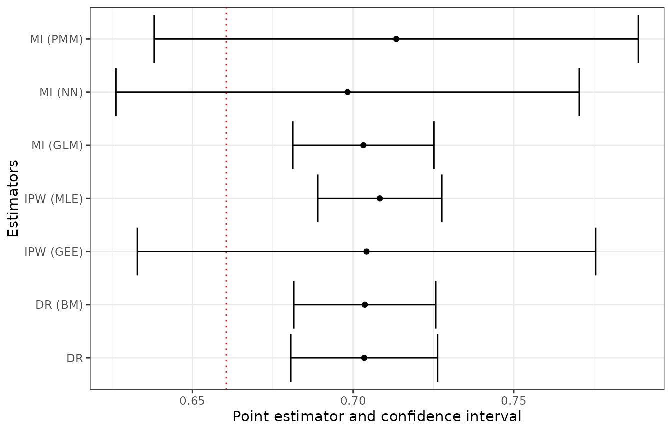

Figure 1: Comparison of estimates of the share of job vacancies offered on a single-shift.

Advanced usage

Bootstrap approach for variance estimation

In the package we allow the user to estimate the variance of the mean analytically (by default) or using the bootstrap approach, as described in the prediction approach section. We use analytical variance estimators proposed in the papers referenced in the methods section. The calculation of the standard error can be disabled using nonprob(se = FALSE). The bootstrap approach implemented in the package refers to:

• the non-probability sample – currently only simple random sampling with replacement is available via the base::sample(),
• the probability sample – all the approaches implemented in the as.svrepdesign() function of the survey package are supported and we refer the reader to the relevant help file.

The bootstrap approach is specified via the control_inf() function with var_method = "bootstrap". The bootstrap method for the probability sample is controlled via the rep_type argument, which passes the method to the as.svrepdesign() function. The number of iterations is set in the num_boot argument (100 by default). If the samples are large or the estimation method is complicated (e.g., involves variable selection) one can set verbose = TRUE to track progress. By default bootstrap results are stored in the boot_sample element of the resulting list (to disable this option, keep_boot should be set to FALSE). The following code is an example of applying the IPW approach with the bootstrap approach specified by the argument control_inference of the nonprob() function.

set.seed(2024)
ipw_est1_boot <- nonprob(
  selection = ~ region + private + nace + size,
  target = ~ single_shift,
  svydesign = jvs_svy,
  data = admin,
  method_selection = "logit",
  control_inference = control_inf(var_method = "bootstrap", num_boot = 50),
  verbose = FALSE
)

Next, we compare the estimated standard error of variance estimation for the analytical and the bootstrap approach.

rbind("IPW analytic variance"  = extract(ipw_est1)[, 2:3],
      "IPW bootstrap variance" = extract(ipw_est1_boot)[, 2:3])
#>                             mean          SE
#> IPW analytic variance  0.7083229 0.009847656
#> IPW bootstrap variance 0.7083229 0.010830659

The boot samples can be accessed via the boot_sample element of the output list of the nonprob() function. Note that the output is returned as a matrix because we allow multiple target variables.

head(ipw_est1_boot$boot_sample, n = 3)
#>      single_shift
#> [1,]    0.7174193
#> [2,]    0.7238239
#> [3,]    0.7249801

Variable selection algorithms

In this section we briefly show how to use variable selection algorithms. In order to indicate that a variable selection algorithm should be used one should specify the control_inference = control_inf(vars_selection = TRUE) argument. Then, the user should either leave the default setting or specify the outcome parameters via the control_out() function or the control_sel() function. Both functions have the same parameters:

• penalty – The penalization function used during variables selection (possible values: c("SCAD", "lasso", "MCP")).
• nlambda – The number of \lambda values; by default set to 50 (grid search).
• lambda_min – The smallest value for \lambda, as a fraction of lambda.max; 0.001 by default.
• lambda – A user specified vector of lambdas (only for the control_sel() function).
• nfolds – The number of folds for cross validation; by default set to 10.
• a_SCAD, a_MCP – The tuning parameter of the SCAD and MCP penalty for the selection model; by default set to 3.7 and 3, respectively.

In the case of the MI approach we rely on the ncvreg package (Breheny and Huang 2011), which is the only R package that employs the SCAD method. For the IPW and DR approaches, we have developed our own codes in C++ via the Rcpp and RcppArmadillo packages. In the code below we apply variable selection for the MI-GLM estimator using only 5 folds, 25 possible values of \lambda parameters and the LASSO penalty.

set.seed(2024)
mi_est1_sel <- nonprob(
  outcome = single_shift ~ region + private + nace + size,
  svydesign = jvs_svy,
  data = admin,
  method_outcome = "glm",
  family_outcome = "binomial",
  control_outcome = control_out(nfolds = 5, nlambda = 25, penalty = "lasso"),
  control_inference = control_inf(vars_selection = TRUE),
  verbose = TRUE
)
#> Starting CV fold #1
#> Starting CV fold #2
#> Starting CV fold #3
#> Starting CV fold #4
#> Starting CV fold #5

In this case study, the MI-GLM estimator with variable selection yields almost the same results as the approach without it. Point estimates and standard errors differ at the fourth and third digit, respectively.

rbind("MI without var sel" = extract(mi_est1)[, 2:3],
      "MI with var sel"    = extract(mi_est1_sel)[, 2:3])
#>                         mean         SE
#> MI without var sel 0.7032089 0.01120237
#> MI with var sel    0.7019291 0.01102109

The result object of the cv.ncvreg class is stored in the "outcome" element of the result, and you can access the selected variables using the coef generic method as follows.

round(coef(mi_est1_sel)$coef_out[, 1], 4)
#> (Intercept)    region04    region06    region08    region10    region12 
#>      0.2820      0.0025      0.3274      0.3196      0.2120      0.1775 
#>    region14    region16    region18    region20    region22    region24 
#>      0.0143      0.0792      0.0000      0.0000      0.0047     -0.2554 
#>    region26    region28    region30    region32     private     naceD.E 
#>      0.1333      0.0000      0.0000      0.0000     -0.6090      0.1759 
#>       naceF       naceG       naceH       naceI       naceJ     naceK.L 
#>      1.9173     -0.4558     -0.5607     -1.0966      0.9214      1.0370 
#>       naceM       naceN       naceO       naceP       naceQ     naceR.S 
#>      1.0025     -0.1840      1.4744      0.5368     -0.7116     -0.8138 
#>       sizeM       sizeS 
#>      0.9972      1.5354

If a user is interested in viewing the PS estimation results, then access to the "selection" element is required.

round(coef(ipw_est1)$coef_sel[, 1], 4)
#> (Intercept)    region04    region06    region08    region10    region12 
#>     -0.6528      0.8378      0.1995      0.1048     -0.1576     -0.6099 
#>    region14    region16    region18    region20    region22    region24 
#>     -0.8415      0.7639      1.1781      0.2225     -0.0375     -0.4067 
#>    region26    region28    region30    region32     private     naceD.E 
#>      0.2029      0.5786     -0.6102      0.3274      0.0590      0.7727 
#>       naceF       naceG       naceH       naceI       naceJ     naceK.L 
#>     -0.3778     -0.3337     -0.6517      0.4118     -1.4264      0.0617 
#>       naceM       naceN       naceO       naceP       naceQ     naceR.S 
#>     -0.4068      0.8003     -0.6935      1.2510      0.3029      0.2223 
#>       sizeM       sizeS 
#>     -0.3641     -1.0292

Classes and S3 methods

The package contains the main class nonprob and the supplementary class nonprob_method and the related nonprob_summary class. All available S3 methods can be obtained by calling methods(class = "nonprob"). For instance, the check_balance() function, already mentioned in the case study, is used to view the balance by checking how the PS weights reproduce known or estimated population totals; the nobs() function returns the sample size of the probability and non-probability samples.

nobs(dr_est1)
#>    prob nonprob 
#>    6523    9344

Table 9 presents S3 methods implemented for objects of class nonprob. We have intentionally limited the number of implemented methods as the goal of the package is to provide point and interval estimates. If users are interested in assessing the quality of the models or the covariate balance, they should use existing R packages.

Table 9. S3 methods implemented for objects of class nonprob in nonprobsvy.

Function	Description
check_balance	Returns a list of totals for IPW and DR estimators.
coef	Returns a list of coefficients for outcome or selection model.
confint	Returns the confidence interval for the target variable(s).
extract	Returns a data.frame with estimation results.
nobs	Returns the number of observations for both samples.
plot	Plots a comparison of naive (uncorrected) and estimated mean along with CI.
pop_size	Returns the population size (fixed or not).
summary	Returns a nonprob_summary class with additional information.
update	Returns an updated object.
weights	Returns IPW weights for the IPW and DR estimator.

The confidence interval for the target variable(s) can be estimated using the generic confint() function.

confint(dr_est1, level = 0.99)
#>         target lower_bound upper_bound
#> 1 single_shift   0.6734503   0.7334886

If a user is interested in assessing the distribution of the IPW weights, we suggest using the weights() function.

summary(weights(dr_est1))
#>    Min. 1st Qu.  Median    Mean 3rd Qu.    Max. 
#>   1.169   2.673   4.333   5.661   7.178  49.950

In the case of mass imputation estimators it is possible to use special functions method_glm() that are of class nonprob_method. An example is given below

res_glm <- method_glm(
  y_nons = admin$single_shift,
  X_nons = model.matrix(~ region + private + nace + size, admin),
  X_rand = model.matrix(~ region + private + nace + size, jvs),
  svydesign = jvs_svy)
res_glm
#> Mass imputation model (GLM approach). Estimated mean: 0.7039 (se: 0.0115)

For the IPW we have created the function method_ps(), which returns requested functions for a specific link. This approach is motivated by the following reasons: 1) we allow different estimation techniques, such as maximum likelihood and general estimation equations; 2) the IPW estimator is also used for the DR estimator; and 3) variance estimators depend on whether the IPW or the DR estimator is applied (with combination with the MI estimator).

method_ps()
#> Propensity score model with logit link

Details can be found in help page.

?method_ps()

Summary and future work

The nonprobsvy package provides a comprehensive R software solution that addresses inference challenges connected with non-probability samples by integrating them with probability samples or known population totals/means. As non-probability data sources, like administrative registers, voluntary online panels, and social media data become increasingly available, statisticians need robust methods to produce reliable population estimates. The package implements state-of-the-art approaches including mass imputation, inverse probability weighting, and doubly robust methods, each designed to correct selection bias by leveraging auxiliary data. By providing a unified framework and its integration with the survey package, the nonprobsvy makes complex statistical methods for non-probability samples more accessible, enabling researchers to produce robust estimates even when working with non-representative data.

There are several avenues for future development of the nonprobsvy package. One key priority is to implement model-based calibration and additional methods for estimating propensity scores and weights. The package currently assumes no overlap between probability and non-probability samples, so accounting for potential overlap (e.g., in big data sources and registers) is another important extension. Additional planned developments include handling non-ignorable sample selection mechanisms, developing a theory for maintaining consistency with calibration weights, and supporting multiple non-probability samples from various sources for the purpose of data integration. Further methodological extensions under consideration include empirical likelihood approaches for doubly/multiply robust estimation, integration of machine learning methods like debiased/double machine learning from causal inference, handling measurement errors in big data variables, and expanding the bootstrap approach beyond simple random sampling with replacement.

The package will also be extended to handle the svyrep.design class from the survey package and the svrep package. These developments will enhance its capabilities for handling complex survey data structures and modern estimation challenges.

Acknowledgements

The authors’ work has been financed by the National Science Centre in Poland, OPUS 20, grant no. 2020/39/B/HS4/00941.

Łukasz Chrostowski was the main developer and maintainer of the package up to version 0.1.0. Parts of this paper are based on Łukasz’s Master’s thesis (available at https://github.com/ncn-foreigners/graduation-theses). Piotr Chlebicki has contributed to the package and has implemented MI-PMM estimators. Maciej Beręsewicz was responsible for the design of the package and for testing, reviewing and contributing to the source code. He also prepared the manuscript. He was also responsible for a significant restructuring of the package between versions 0.1.0 and 0.2.0.

The authors thank editors and reviewers for their constructive suggestions.

Appendix: Algorithms for the MI-NN and MI-PMM estimators

Algorithm 1. Mass imputation using the k nearest neighbor algorithm.

1. If k=1, then for each i \in S_{\text{P}} match \hat{\nu}(i) such that \hat{\nu}(i)=\operatorname{arg\,min}_{j\in S_{\text{NP}}}d\left(\boldsymbol{x}_i,\boldsymbol{x}_j\right).
2. If k>1, then \hat{\nu}(i, z) = \operatorname{arg\,min}_{j\in S_{\text{NP}}\setminus\bigcup_{t=1}^{z-1}\{\hat{\nu}(i, t)\}} d\left(\boldsymbol{x}_i, \boldsymbol{x}_j\right), i.e., \hat{\nu}(i, z) is z-th nearest neighbor from the sample S_{\text{NP}}.
3. For each i \in S_{\text{P}}, calculate the imputed value as y_i^* = \frac{1}{k}\sum_{t=1}^{k}y_{\hat{\nu}(i, t)}.

Algorithm 2. Mass imputation using predictive mean matching variant: \hat{y}-\hat{y} matching.

1. Estimate regression model m(\boldsymbol{x}, \boldsymbol{\beta}) parameters.
2. Predict \hat{y}_{i}=m\left(\boldsymbol{x}_{i}, \hat{\boldsymbol{\beta}}\right), \hat{y}_{j}=m\left(\boldsymbol{x}_{j}, \hat{\boldsymbol{\beta}}\right) for i\in S_{\text{P}}, j\in S_{\text{NP}} and assign each i\in S_{\text{P}} to \hat{\nu}(i), where \hat{\nu}(i)=\operatorname{arg\,min}_{j\in S_{\text{NP}}}d\left(\hat{y}_{i}, \hat{y}_{j}\right).
3. If k>1, then \hat{\nu}(i, z) = \operatorname{arg\,min}_{j\in S_{\text{NP}}\setminus\bigcup_{t=1}^{z-1}\{\hat{\nu}(i, t)\}} d\left(\hat{y}_{i}, \hat{y}_{j}\right), e.g., \hat{\nu}(i, z) is z-th nearest neighbor from a sample S_{\text{NP}}.
4. For i \in S_{\text{P}}, calculate imputation value as y_i^* = \frac{1}{k}\sum_{t=1}^{k}y_{\hat{\nu}(i, t)}.

Algorithm 3. Mass imputation using predictive mean matching variant: \hat{y}-y matching.

1. Estimate regression model m(\boldsymbol{x}, \boldsymbol{\beta}) parameters.
2. Predict \hat{y}_{i}=m\left(\boldsymbol{x}_{i}, \hat{\boldsymbol{\beta}}\right) for i \in S_{\text{P}} and assign each i \in S_{\text{P}} to \hat{\nu}(i), where \hat{\nu}(i)=\operatorname{arg\,min}_{j \in S_{\text{NP}}}d\left(\hat{y}_{i}, y_{j}\right).
3. If k>1, then \hat{\nu}(i, z) = \operatorname{arg\,min}_{j \in S_{\text{NP}} \setminus \bigcup_{t=1}^{z-1}\{\hat{\nu}(i, t)\}} d\left(\hat{y}_{i}, y_{j}\right).
4. For each i \in S_{\text{P}} calculate imputation value as y_i^* = \frac{1}{k}\sum_{t=1}^{k}y_{\hat{\nu}(i, t)}.

References

Abadie, Alberto, and Guido W Imbens. 2006. “Large Sample Properties of Matching Estimators for Average Treatment Effects.” Econometrica 74 (1): 235–67. https://doi.org/10.1111/j.1468-0262.2006.00655.x.

Beaumont, Jean-Francois. 2020. “Are Probability Surveys Bound to Disappear for the Production of Official Statistics.” Survey Methodology 46 (1): 1–28. https://doi.org/10.4135/9781452226620.n14.

Beręsewicz, Maciej. 2017. “A Two-Step Procedure to Measure Representativeness of Internet Data Sources.” International Statistical Review 85 (3): 473–93. https://doi.org/10.1111/insr.12217.

Beręsewicz, Maciej, Marcin Szymkowiak, and Piotr Chlebicki. 2025. “Quantile Balancing Inverse Probability Weighting for Non-Probability Samples.” Survey Methodology 51 (2): 1–25.

Bezanson, Jeff, Alan Edelman, Stefan Karpinski, and Viral B. Shah. 2017. “: A Fresh Approach to Numerical Computing.” SIAM Review 59 (1): 65–98. https://doi.org/10.1137/141000671.

Biffignandi, Silvia, and Jelke Bethlehem. 2021. Handbook of Web Surveys. 1st ed. John Wiley & Sons. https://doi.org/10.1002/9781119371717.

Breheny, Patrick, and Jian Huang. 2011. “Coordinate Descent Algorithms for Nonconvex Penalized Regression, with Applications to Biological Feature Selection.” The Annals of Applied Statistics 5 (1): 232–53. https://doi.org/10.1214/10-aoas388.

Carpenter, Bob, Andrew Gelman, Matthew D Hoffman, et al. 2017. “: A Probabilistic Programming Language.” Journal of Statistical Software 76: 1–32. https://doi.org/10.18637/jss.v076.i01.

Castro, Luis Mart’ın. 2024. : Inference from Non-Probability Samples. https://pypi.org/project/inps/.

Chen, Jack, Richard Valliant, and Michael Elliott. 2018. “Model-Assisted Calibration of Non-Probability Sample Survey Data Using Adaptive LASSO.” Survey Methodology 44 (1): 117–44. https://doi.org/10.1111/rssc.12327.

Chen, Sixia, Shu Yang, and Jae Kwang Kim. 2022. “Nonparametric Mass Imputation for Data Integration.” Journal of Survey Statistics and Methodology 10 (1): 1–24. https://doi.org/10.1093/jssam/smaa036.

Chen, Yilin, Pengfei Li, and Changbao Wu. 2020. “Doubly Robust Inference with Nonprobability Survey Samples.” Journal of the American Statistical Association 115 (532): 2011–21. https://doi.org/10.1080/01621459.2019.1677241.

Chlebicki, Piotr, Łukasz Chrostowski, and Maciej Beręsewicz. 2024. Data Integration of Non-Probability and Probability Samples with Predictive Mean Matching. arXiv 2403.13750. arXiv.org E-Print Archive. https://doi.org/10.48550/arXiv.2403.13750.

Chrostowski, Łukasz. 2024. “Statistical Inference with Non-Probability Samples.” Master’s thesis, Adam Mickiewicz University. https://github.com/ncn-foreigners/graduation-theses/blob/main/2024-Chrostowski.pdf.

Chrostowski, Łukasz, Maciej Beręsewicz, and Piotr Chlebicki. 2025. Inference Based on Non-Probability Samples. https://github.com/ncn-foreigners/nonprobsvy.

Citro, Constance F. 2014. “From Multiple Modes for Surveys to Multiple Data Sources for Estimates.” Survey Methodology 40 (2): 137–62.

Cobo, Beatriz, Ram’on Ferri-Garc’ıa, Jorge L. Rueda-S’anchez, and Mar’ıa del Mar Rueda. 2024. “Software Review for Inference with Non-Probability Surveys.” The Survey Statistician 90: 40–47. https://doi.org/10.1016/j.matcom.2024.08.009.

Daas, Piet JH, Marco J Puts, Bart Buelens, and Paul AM van den Hurk. 2015. “Big Data as a Source for Official Statistics.” Journal of Official Statistics 31 (2): 249–62. https://doi.org/10.1515/jos-2015-0016.

Diallo, Mamadou S. 2021. “: A Package for Selecting, Weighting and Analyzing Data from Complex Sampling Designs.” Journal of Open Source Software 6 (68): 3376. https://doi.org/10.21105/joss.03376.

Elliott, Michael R., and Richard Valliant. 2017. “Inference for Nonprobability Samples.” Statistical Science 32 (2): 237–64. https://doi.org/10.1214/16-sts598.

Fjelde, Tor Erlend, Kai Xu, David Widmann, et al. 2025. “: A General-Purpose Probabilistic Programming Language.” ACM Trans. Probab. Mach. Learn. (New York, NY, USA), ahead of print. https://doi.org/10.1145/3711897.

Gelman, Andrew. 1997. “Poststratification into Many Categories Using Hierarchical Logistic Regression.” Survey Methodology 23: 127–35. https://doi.org/10.11126/stanford/9780804753005.003.0011.

Goodrich, Ben, Jonah Gabry, Imad Ali, and Sam Brilleman. 2024. : Bayesian Applied Regression Modeling via . https://mc-stan.org/rstanarm/.

Greifer, Noah. 2024. : Covariate Balance Tables and Plots. https://doi.org/10.32614/CRAN.package.cobalt.

Grow, Andr’e, Daniela Perrotta, Emanuele Del Fava, et al. 2022. “Is Facebook’s Advertising Data Accurate Enough for Use in Social Science Research? Insights from a Cross-National Online Survey.” Journal of the Royal Statistical Society A 185 (2): 343–63. https://doi.org/10.1111/rssa.12948.

Hayfield, Tristen, and Jeffrey S. Racine. 2008. “Nonparametric Econometrics: The Package.” Journal of Statistical Software 27 (5): 1–32. https://doi.org/10.18637/jss.v027.i05.

Institute Inc. 2023. Software, Version 9.4. Cary, NC. https://www.sas.com/.

Jefferis, Gregory, Samuel E. Kemp, Sunil Arya, and David Mount. 2024. : Fast Nearest Neighbour Search (Wraps ANN Library) Using L2 Metric. https://doi.org/10.32614/CRAN.package.RANN.

Kim, Jae Kwang, and David Haziza. 2014. “Doubly Robust Inference with Missing Data in Survey Sampling.” Statistica Sinica 24 (1): 375–94. https://doi.org/10.5705/ss.2012.005.

Kim, Jae Kwang, and Kento Morikawa. 2023. “An Empirical Likelihood Approach to Reduce Selection Bias in Voluntary Samples.” Calcutta Statistical Association Bulletin 75 (1): 8–27. https://doi.org/10.1177/00080683231186488.

Kim, Jae Kwang, Seho Park, Yilin Chen, and Changbao Wu. 2021. “Combining Non-Probability and Probability Survey Samples Through Mass Imputation.” Journal of the Royal Statistical Society A 184 (3): 941–63. https://doi.org/10.1111/rssa.12696.

Kim, Jae Kwang, and Minsun Kim Riddles. 2012. “Some Theory for Propensity-Score-Adjustment Estimators in Survey Sampling.” Survey Methodology 38 (2): 157–65. https://doi.org/10.1093/jssam/smv047.

Lee, Sunghee. 2006. “Propensity Score Adjustment as a Weighting Scheme for Volunteer Panel Web Surveys.” Journal of Official Statistics 22 (2): 329. https://doi.org/10.1177/0049124108329643.

Lee, Sunghee, and Richard Valliant. 2009. “Estimation for Volunteer Panel Web Surveys Using Propensity Score Adjustment and Calibration Adjustment.” Sociological Methods & Research 37 (3): 319–43. https://doi.org/10.1177/0049124108329643.

Lohr, Sharon L. 2021. Software Companion for Sampling: Design and Analysis. 3rd ed. Chapman; Hall/CRC. https://doi.org/10.1201/9781003160366.

Lumley, Thomas. 2004. “Analysis of Complex Survey Samples.” Journal of Statistical Software 9 (1): 1–19. https://doi.org/10.18637/jss.v009.i08.

Mart’ın, Luis Castro, Ram’on Ferri Garc’ıa, and Mar’ıa del Mar Rueda. 2020. : Estimation in Nonprobability Sampling. https://doi.org/10.32614/CRAN.package.nonprobest.

Meng, Xiao-Li. 2018. “Statistical Paradises and Paradoxes in Big Data (I): Law of Large Populations, Big Data Paradox, and the 2016 US Presidential Election.” The Annals of Applied Statistics 12: 685–726. https://doi.org/10.1214/18-aoas1161sf.

Rivers, Douglas. 2007. “Sampling for Web Surveys.” Proceedings of the Survey Research Methods Section, Joint Statistical Meetings (Alexandria, VA), 1–26.

Robins, James M, Andrea Rotnitzky, and Lue Ping Zhao. 1994. “Estimation of Regression Coefficients When Some Regressors Are Not Always Observed.” Journal of the American Statistical Association 89 (427): 846–66. https://doi.org/10.1080/01621459.1994.10476818.

Sarig, Tal, Tal Galili, and Roee Eilat. 2023. – a Package for Balancing Biased Data Samples. arXiv 2307.06024. arXiv.org E-Print Archive. https://doi.org/10.48550/arXiv.2307.06024.

Särndal, Carl-Erik, and Sixten Lundström. 2005. Estimation in Surveys with Nonresponse. 1st ed. John Wiley & Sons. https://doi.org/10.1002/0470011351.

Schonlau, Matthias, and Mick P Couper. 2017. “Options for Conducting Web Surveys.” Statistical Science 32 (2): 279–92. https://doi.org/10.1214/16-sts597.

StataCorp. 2025. Statistical Software: Release 19. StataCorp LLC.

Statistics Poland. 2021. The Demand for Labour: Methodological Report. Statistical Office in Bydgoszcz. https://stat.gov.pl/obszary-tematyczne/rynek-pracy/popyt-na-prace/zeszyt-metodologiczny-popyt-na-prace,3,1.html.

Tibshirani, Robert. 1996. “Regression Shrinkage and Selection via the Lasso.” Journal of the Royal Statistical Society B 58 (1): 267–88. https://doi.org/10.1111/j.2517-6161.1996.tb02080.x.

Valliant, Richard, and Jill A Dever. 2018. Survey Weights: A Step-by-Step Guide to Calculation. Vol. 1. Stata Press.

van Buuren, Stef, and Karin Groothuis-Oudshoorn. 2011. “: Multivariate Imputation by Chained Equations in .” Journal of Statistical Software 45 (3): 1–67. https://doi.org/10.18637/jss.v045.i03.

Virtanen, Pauli, Ralf Gommers, Travis E. Oliphant, et al. 2020. “ 1.0: Fundamental Algorithms for Scientific Computing in .” Nature Methods 17: 261–72. https://doi.org/10.1038/s41592-019-0686-2.

Wand, Matt. 2025. : Functions for Kernel Smoothing Supporting Wand and Jones (1995). https://doi.org/10.32614/CRAN.package.kernsmooth.

Wu, Changbao. 2022. “Statistical Inference with Non-Probability Survey Samples.” Survey Methodology 48: 283–311. https://doi.org/10.1002/9780470191590.ch10.

Yang, Shu, and Jae Kwang Kim. 2020. “Asymptotic Theory and Inference of Predictive Mean Matching Imputation Using a Superpopulation Model Framework.” Scandinavian Journal of Statistics 47 (3): 839–61. https://doi.org/10.1111/sjos.12429.

Yang, Shu, Jae Kwang Kim, and Rui Song. 2020. “Doubly Robust Inference When Combining Probability and Non-Probability Samples with High Dimensional Data.” Journal of the Royal Statistical Society B 82 (2): 445–65. https://doi.org/10.1111/rssb.12354.

Yang, Shu, Jae-Kwang Kim, and Youngdeok Hwang. 2021. “Integration of Data from Probability Surveys and Big Found Data for Finite Population Inference Using Mass Imputation.” Survey Methodology 47 (1): 29–58. https://doi.org/10.46852/0424-2513.3.2024.10.