Balancing distributions for observational studies
Maciej Beręsewicz
Source:vignettes/d_causal.Rmd
d_causal.RmdTheory
Distributional entropy balancing
Our proposal, which leads to distributional entropy balancing (hereinafter DEB), is based on extending the original idea by adding additional constraint(s) on the weights on , as presented below.
Distributional propensity score method
(imai2014covariate?) proposed covariate balancing propensity score (CBPS) to estimate the (eqref?){eq-ate}, where unknown parameters of the propensity score model are estimated using the generalized method of moments as
where is the propensity score. This balances means of the the variables, which may not be sufficient if the variables are highly skewed or we are interested in estimating DTE or QTE.
We propose a simple approach based on the specification of moments and -quantiles to be balanced. Instead of using the matrix , we propose to use the matrix , which is constructed as follows
where are matrices of size and with covariates to be balanced at the means, and are matrices with are based on covariates with elements defined as follows
and
where is the size of the treatment group, or alternatively the logistic function can be used.
Packages
Load packages for the example
library(jointCalib)
library(CBPS)
#> Loading required package: MASS
#> Loading required package: MatchIt
#> Loading required package: nnet
#> Loading required package: numDeriv
#> Loading required package: glmnet
#> Loading required package: Matrix
#> Loaded glmnet 4.1-8
#> CBPS: Covariate Balancing Propensity Score
#> Version: 0.23
#> Authors: Christian Fong [aut, cre],
#>   Marc Ratkovic [aut],
#>   Kosuke Imai [aut],
#>   Chad Hazlett [ctb],
#>   Xiaolin Yang [ctb],
#>   Sida Peng [ctb],
#>   Inbeom Lee [ctb]
library(ebal)
#> ##
#> ## ebal Package: Implements Entropy Balancing.
#> ## See http://www.stanford.edu/~jhain/ for additional information.
library(laeken)
Read the the LaLonde data from the CBPS
package.
data("LaLonde", package = "CBPS")
head(LaLonde)
#>     exper treat age educ black hisp married nodegr re74 re75 re78 re74.miss
#> 298     0     0  47   12     0    0       0      0    0    0    0         0
#> 299     0     0  50   12     1    0       1      0    0    0    0         1
#> 300     0     0  44   12     0    0       0      0    0    0    0         0
#> 301     0     0  28   12     1    0       1      0    0    0    0         1
#> 302     0     0  54   12     0    0       1      0    0    0    0         1
#> 303     0     0  55   12     0    1       1      0    0    0    0         1
ATT with entropy balancing and other methods
Single variable: age
First, we start with the age variable. Below we can find
the distribution of age in the control and treatment group.
dens0 <- density(LaLonde$age[LaLonde$treat == 0])
dens1 <- density(LaLonde$age[LaLonde$treat == 1])
plot(dens0, main="Distribution of age", xlab="Age", ylim=c(0, max(dens0$y, dens1$y)), col = "blue")
lines(dens1, lty=2, col="red")
legend("topright", legend=c("Control", "Treatment"), lty=c(1,2), col=c("blue", "red"))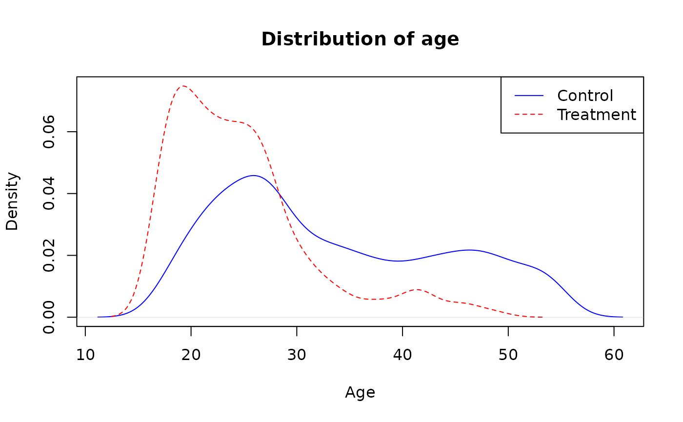
Basic descriptive statistics are given below.
aggregate(age ~ treat, data = LaLonde, FUN = quantile)
#>   treat age.0% age.25% age.50% age.75% age.100%
#> 1     0   17.0    25.0    31.0    42.5     55.0
#> 2     1   17.0    20.0    23.0    27.0     49.0
Nowe, let’s use ebal::ebalance and
jointCalib::joint_calib_att with method eb (it
uses uses ebal package as backend). For DEB we use deciles
probs = seq(0.1, 0.9, 0.1) and balance mean as well
(formula_means = ~ age). The output informs that about the
target (totals) quantiles and difference between balanced
and the target quantities (column precision).
bal_standard <- ebalance(LaLonde$treat, X = LaLonde[, "age"])
#> Converged within tolerance
bal_quant <- joint_calib_att(formula_means = ~ age,
                             formula_quantiles = ~ age,
                             treatment =  ~ treat,
                             data = LaLonde,
                             probs = seq(0.1, 0.9, 0.1),
                             method = "eb")
bal_quant
#> Weights calibrated using: eb with ebal backend.
#> Summary statistics for g-weights:
#>     Min.  1st Qu.   Median     Mean  3rd Qu.     Max.
#> 0.007665 0.022555 0.046914 0.101888 0.194177 0.605874
#> Totals and precision (abs diff: 0.1299956)
#>          totals    precision
#> N         297.0 2.632778e-03
#> age 0.10    0.1 1.688971e-10
#> age 0.20    0.2 3.377949e-10
#> age 0.30    0.3 5.067252e-10
#> age 0.40    0.4 3.901260e-09
#> age 0.50    0.5 6.496022e-09
#> age 0.60    0.6 1.144491e-08
#> age 0.70    0.7 3.277056e-08
#> age 0.80    0.8 5.172449e-08
#> age 0.90    0.9 1.811425e-07
#> age      7314.0 1.273625e-01
Compare weighted distributions with treatment group distribution.
dens0 <- density(LaLonde$age[LaLonde$treat == 0], weights = bal_standard$w/sum(bal_standard$w))
#> Warning in density.default(LaLonde$age[LaLonde$treat == 0], weights =
#> bal_standard$w/sum(bal_standard$w)): Selecting bandwidth *not* using 'weights'
dens1 <- density(LaLonde$age[LaLonde$treat == 0], weights = bal_quant$g/sum(bal_quant$g))
#> Warning in density.default(LaLonde$age[LaLonde$treat == 0], weights =
#> bal_quant$g/sum(bal_quant$g)): Selecting bandwidth *not* using 'weights'
dens2 <- density(LaLonde$age[LaLonde$treat == 1])
plot(dens0, main="Distribution of age", xlab="Age", ylim=c(0, max(dens0$y, dens1$y)))
lines(dens1, lty=2, col="blue")
lines(dens2, lty=3, col="red")
legend("topright",
       legend=c("EB", "DEB", "Treatment"),
       lty=c(1,2, 3),
       col=c("black", "blue", "red"))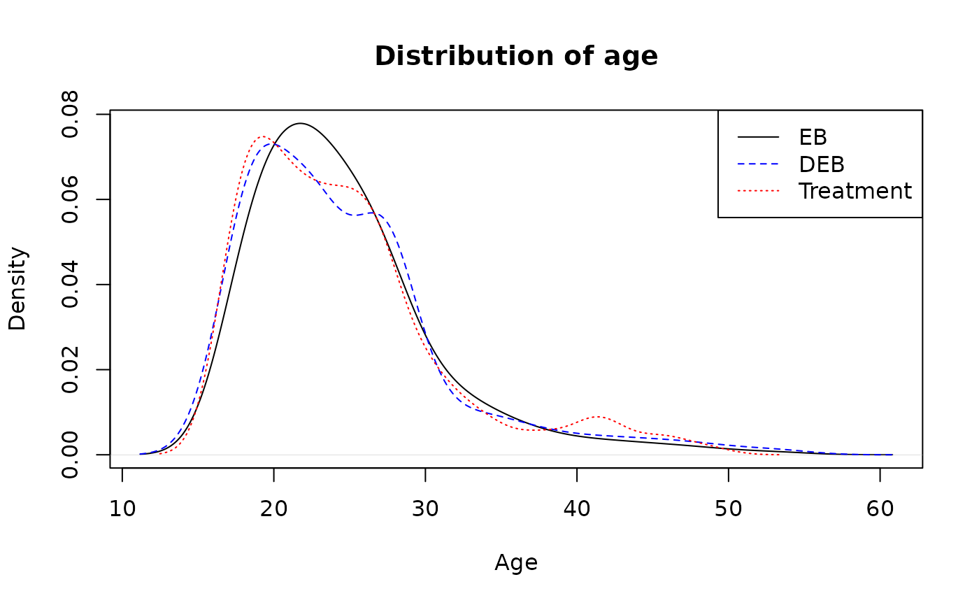
Compare balancing weights.
plot(x = bal_standard$w,
     y = bal_quant$g,
     xlab = "EB", ylab = "DEB", main = "Comparison of EB and DEB weights",
     xlim = c(0, 0.7), ylim = c(0, 0.7))
More variables
Now, consider three variables: married, age
and educ.
dens0 <- density(LaLonde$educ[LaLonde$treat == 0])
dens1 <- density(LaLonde$educ[LaLonde$treat == 1])
plot(dens0, main="Distribution of education", xlab="Education", ylim=c(0, max(dens0$y, dens1$y)), col = "blue")
lines(dens1, lty=2, col="red")
legend("topleft", legend=c("Control", "Treatment"), lty=c(1,2), col=c("blue", "red"))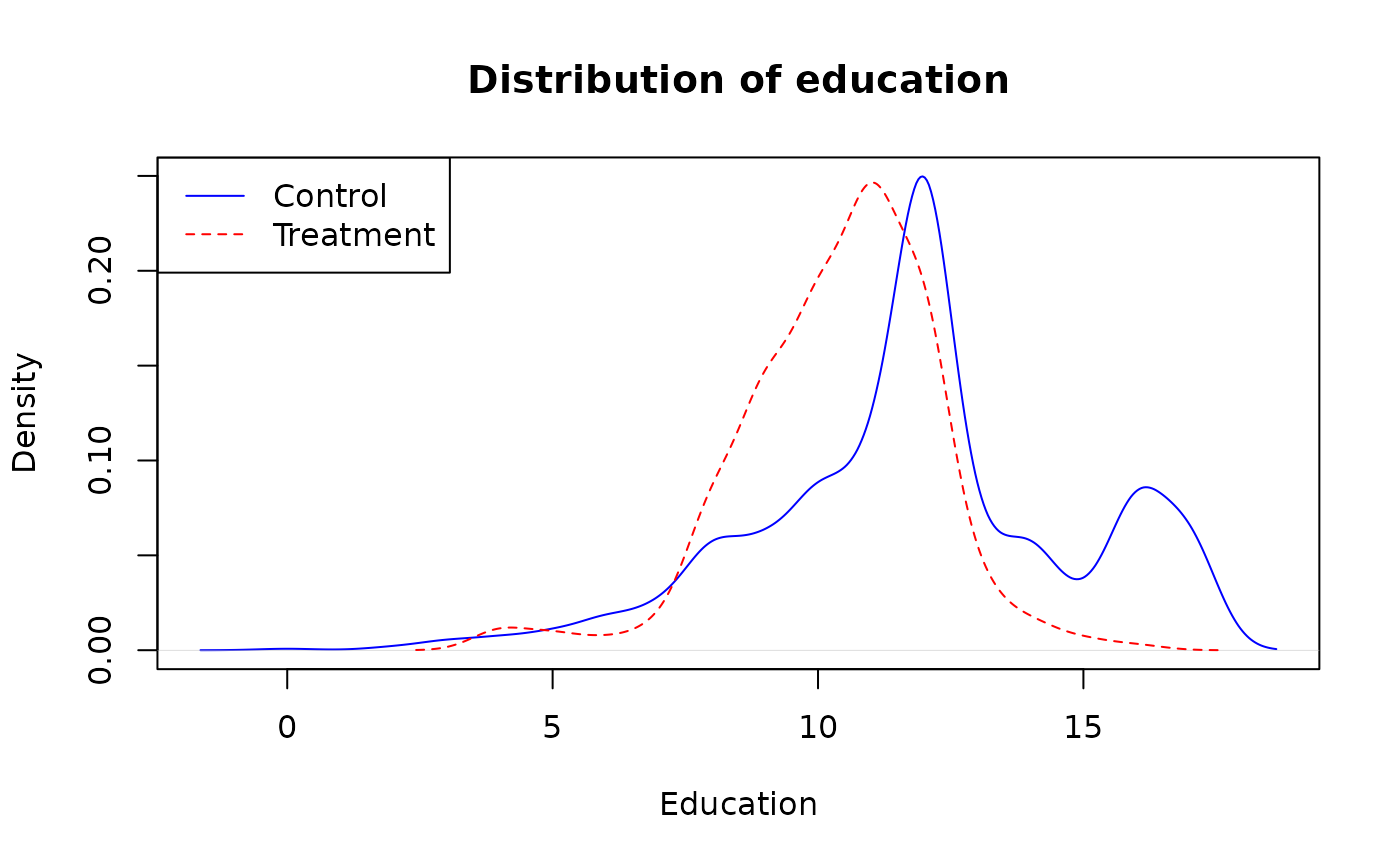
The code below balances control and treatment group on age and educ means and quantiles.
bal_standard <- ebalance(LaLonde$treat, X = LaLonde[, c("married", "age", "educ")])
#> Converged within tolerance
bal_quant <- joint_calib_att(formula_means = ~ married + age + educ,
                             formula_quantiles = ~ age + educ,
                             treatment =  ~ treat,
                             data = LaLonde,
                             method = "eb")
bal_quant
#> Weights calibrated using: eb with ebal backend.
#> Summary statistics for g-weights:
#>      Min.   1st Qu.    Median      Mean   3rd Qu.      Max.
#> 0.0003863 0.0075341 0.0258057 0.1018874 0.0606804 2.8081281
#> Totals and precision (abs diff: 0.08993871)
#>            totals    precision
#> N          297.00 1.646454e-03
#> age 0.25     0.25 6.697795e-08
#> age 0.50     0.50 1.541813e-07
#> age 0.75     0.75 4.802355e-07
#> educ 0.25    0.25 2.806495e-06
#> educ 0.50    0.50 3.414877e-06
#> educ 0.75    0.75 4.188730e-06
#> married     50.00 8.466613e-04
#> age       7314.00 7.261357e-02
#> educ      3083.00 1.482091e-02
Compare distribution education (educ) variable.
dens0 <- density(LaLonde$educ[LaLonde$treat == 0], weights = bal_standard$w/sum(bal_standard$w))
#> Warning in density.default(LaLonde$educ[LaLonde$treat == 0], weights =
#> bal_standard$w/sum(bal_standard$w)): Selecting bandwidth *not* using 'weights'
dens1 <- density(LaLonde$educ[LaLonde$treat == 0], weights = bal_quant$g/sum(bal_quant$g))
#> Warning in density.default(LaLonde$educ[LaLonde$treat == 0], weights =
#> bal_quant$g/sum(bal_quant$g)): Selecting bandwidth *not* using 'weights'
dens2 <- density(LaLonde$educ[LaLonde$treat == 1])
plot(dens0, main="Distribution of Education", xlab="Education", ylim=c(0, max(dens0$y, dens1$y)))
lines(dens1, lty=2, col="blue")
lines(dens2, lty=3, col="red")
legend("topleft",
       legend=c("EB", "DEB", "Treatment"),
       lty=c(1,2, 3),
       col=c("black", "blue", "red"))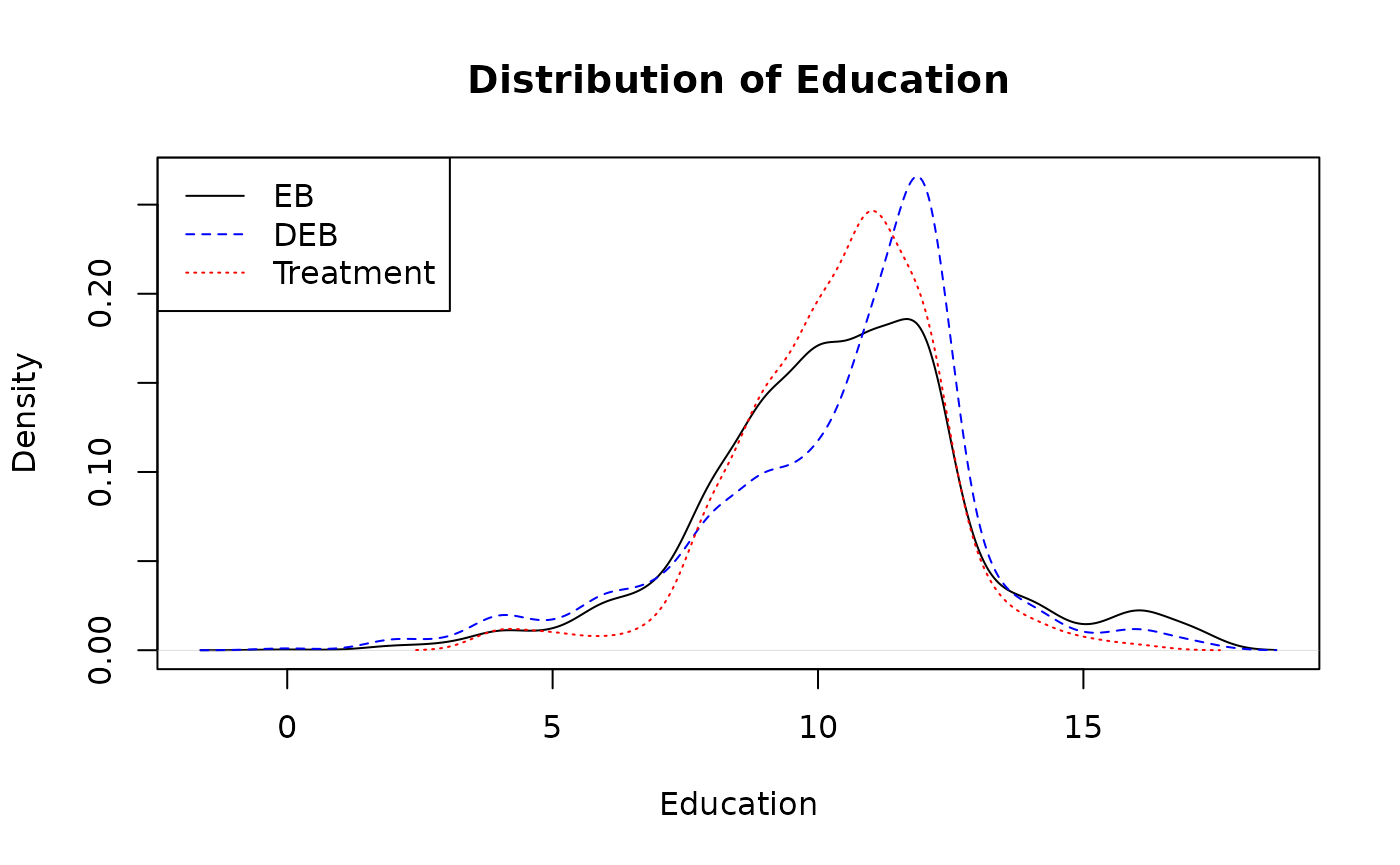
Compare distribution age (age) variable.
dens0 <- density(LaLonde$age[LaLonde$treat == 0], weights = bal_standard$w/sum(bal_standard$w))
#> Warning in density.default(LaLonde$age[LaLonde$treat == 0], weights =
#> bal_standard$w/sum(bal_standard$w)): Selecting bandwidth *not* using 'weights'
dens1 <- density(LaLonde$age[LaLonde$treat == 0], weights = bal_quant$g/sum(bal_quant$g))
#> Warning in density.default(LaLonde$age[LaLonde$treat == 0], weights =
#> bal_quant$g/sum(bal_quant$g)): Selecting bandwidth *not* using 'weights'
dens2 <- density(LaLonde$age[LaLonde$treat == 1])
plot(dens0, main="Distribution of age", xlab="Age", ylim=c(0, max(dens0$y, dens1$y)))
lines(dens1, lty=2, col="blue")
lines(dens2, lty=3, col="red")
legend("topright",
       legend=c("EB", "DEB", "Treatment"),
       lty=c(1,2, 3),
       col=c("black", "blue", "red"))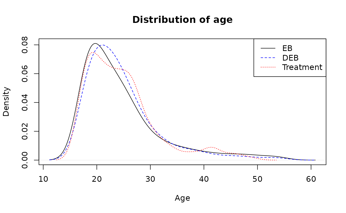
Compare balancing weights.
plot(x = bal_standard$w,
     y = bal_quant$g,
     xlab = "EB", ylab = "DEB", main = "Comparison of EB and DEB weights",
     xlim = c(0, 3), ylim = c(0, 3))
More variables: all variables
Now consider all variables available in the LaLonde
dataset.
bal_standard <- ebalance(LaLonde$treat,
                         X = model.matrix(~ -1 + age + educ + black + hisp + married + nodegr + re74 + re75,
                                          LaLonde))
#> Converged within tolerance

bal_quant <- joint_calib_att(formula_means = ~ age + educ + black + hisp + married + nodegr + re74 + re75,
                             formula_quantiles = ~ age + re74 + re75,
                             probs = 0.5,
                             treatment =  ~ treat,
                             data = LaLonde,
                             method = "eb")
bal_quant
#> Weights calibrated using: eb with ebal backend.
#> Summary statistics for g-weights:
#>     Min.  1st Qu.   Median     Mean  3rd Qu.     Max.
#> 0.000000 0.003086 0.013909 0.101887 0.065794 1.154954
#> Totals and precision (abs diff: 0.03793366)
#>              totals    precision
#> N             297.0 1.080405e-06
#> age 0.50        0.5 8.307879e-10
#> re74 0.50       0.5 1.459702e-10
#> re75 0.50       0.5 4.480682e-11
#> age          7314.0 3.147376e-05
#> educ         3083.0 1.304752e-05
#> black         238.0 5.857759e-07
#> hisp           28.0 5.359394e-08
#> married        50.0 5.735294e-07
#> nodegr        217.0 3.585783e-07
#> re74      1060586.7 1.832775e-02
#> re75       910631.2 1.955873e-02
Compare re74
dens0 <- density(LaLonde$re74[LaLonde$treat == 0], weights = bal_standard$w/sum(bal_standard$w))
#> Warning in density.default(LaLonde$re74[LaLonde$treat == 0], weights =
#> bal_standard$w/sum(bal_standard$w)): Selecting bandwidth *not* using 'weights'
dens1 <- density(LaLonde$re74[LaLonde$treat == 0], weights = bal_quant$g/sum(bal_quant$g))
#> Warning in density.default(LaLonde$re74[LaLonde$treat == 0], weights =
#> bal_quant$g/sum(bal_quant$g)): Selecting bandwidth *not* using 'weights'
dens2 <- density(LaLonde$re74[LaLonde$treat == 1])
plot(dens0, main="Distribution of re74", xlab="Age", ylim=c(0, max(dens0$y, dens1$y)))
lines(dens1, lty=2, col="blue")
lines(dens2, lty=3, col="red")
legend("topright",
       legend=c("EB", "DEB", "Treatment"),
       lty=c(1,2, 3),
       col=c("black", "blue", "red"))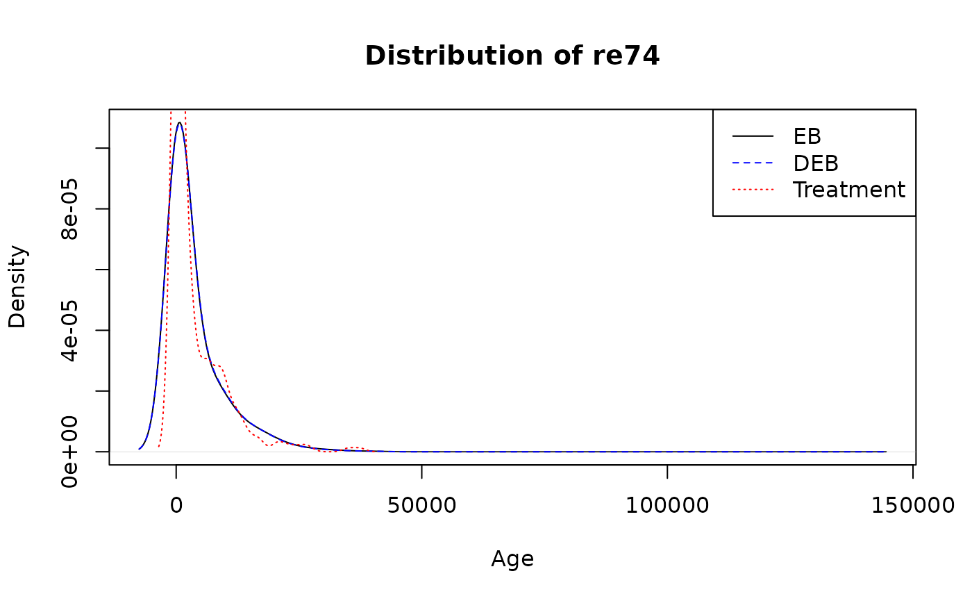
Compare balancing weights.
plot(x = bal_standard$w,
     y = bal_quant$g,
     xlab = "EB", ylab = "DEB", main = "Comparison of EB and DEB weights",
     xlim = c(0, 1.2), ylim = c(0, 1.2))
Compare estimates of ATT using EB and DEB.
c(EB = with(LaLonde, mean(re78[treat == 1]) - weighted.mean(re78[treat == 0], bal_standard$w)),
  DEB = with(LaLonde, mean(re78[treat == 1]) - weighted.mean(re78[treat == 0], bal_quant$g)))
#>        EB       DEB
#> -378.4217 -392.0171
Compare QTT(0.5) using EB and DEB.
c(EB = with(LaLonde, median(re78[treat == 1]) - weightedMedian(re78[treat == 0], bal_standard$w)),
  DEB = with(LaLonde, median(re78[treat == 1]) - weightedMedian(re78[treat == 0], bal_quant$g)))
#>       EB      DEB
#> 72.39014 35.93408
Compare QTT() where .
probs_qtt <- seq(0.1, 0.9, 0.1)
data.frame(
  EB = with(LaLonde,
            quantile(re78[treat == 1], probs_qtt) - weightedQuantile(re78[treat == 0], bal_standard$w, probs_qtt)),
  DEB = with(LaLonde,
            quantile(re78[treat == 1], probs_qtt) - weightedQuantile(re78[treat == 0], bal_quant$g, probs_qtt))
)
#>              EB         DEB
#> 10%     0.00000     0.00000
#> 20%     0.00000     0.00000
#> 30%   788.12509   784.81613
#> 40%   265.73521   261.63315
#> 50%    72.39014    35.93408
#> 60%   156.65605   -20.31025
#> 70%  -549.49531  -669.21504
#> 80%  -498.36777  -498.36777
#> 90% -2818.06621 -2818.06621
ATT with CBPS and DPS [work in progress]
m0 <- CBPS(formula = treat ~ age + educ + black + hisp + married + nodegr + re74,
           data = LaLonde)
#> [1] "Finding ATT with T=1 as the treatment.  Set ATT=2 to find ATT with T=0 as the treatment"
m1 <- joint_calib_cbps(formula_means = ~ age + educ + black + hisp + married + nodegr,
                       formula_quantiles = ~ re74,
                       probs = 0.5,
                       treatment =  ~ treat,
                       data = LaLonde)