Setup
Read required packages
library(blocking)
library(data.table)
#>
#> Attaching package: 'data.table'
#> The following object is masked from 'package:base':
#>
#>     %notin%
Data
Read the example data from the tutorial on the
reclin package on the URos 2021 Conference. The data
sets are from ESSnet on Data Integration as stated in the
repository:
These totally fictional data sets are supposed to have captured details of
persons up to the date 31 December 2011.  Any years of birth captured as 2012
are therefore in error.  Note that in the fictional Census data set, dates of
birth between 27 March 2011 and 31 December 2011 are not necessarily in error.

census: A fictional data set to represent some observations from a
        decennial Census
cis: Fictional observations from Customer Information System, which is
        combined administrative data from the tax and benefit systems

In the dataset census all records contain a person_id. For some of the records
in cis the person_id is also available. This information can be used to
evaluate the linkage (assuming these records from the cis are representable
all records in the cis). -
censusobject has 25343 rows and 13 columns, -
cisobject has 24613 rows and 10 columns.
Census data
head(census)
#>       person_id pername1 pername2    sex dob_day dob_mon dob_year hse_num
#>          <char>   <char>   <char> <char>  <char>  <char>   <char>   <num>
#> 1: DE03US001001    COUIE    PRICE      M       1       6     1960       1
#> 2: DE03US001002    ABBIE    PVICE      F       9      11     1961       1
#> 3: DE03US001003    LACEY    PRICE      F       7       2     1999       1
#> 4: DE03US001004   SAMUEL    PRICE      M      13       4     1990       1
#> 5: DE03US001005   JOSEPH    PRICE      M      20       4     1986       1
#> 6: DE03US001006     JOSH    PRICE      M      14       2     1996       1
#>           enumcap enumpc      str_nam         cap_add        census_id
#>            <char> <char>       <char>          <char>           <char>
#> 1: 1 WINDSOR ROAD DE03US Windsor Road 1, Windsor Road CENSDE03US001001
#> 2: 1 WINDSOR ROAD DE03US Windsor Road 1, Windsor Road CENSDE03US001002
#> 3: 1 WINDSOR ROAD DE03US Windsor Road 1, Windsor Road CENSDE03US001003
#> 4: 1 WINDSOR ROAD DE03US Windsor Road 1, Windsor Road CENSDE03US001004
#> 5: 1 WINDSOR ROAD DE03US Windsor Road 1, Windsor Road CENSDE03US001005
#> 6: 1 WINDSOR ROAD DE03US Windsor Road 1, Windsor Road CENSDE03US001006
CIS data
head(cis)
#>        person_id pername1 pername2    sex dob_day dob_mon dob_year
#>           <char>   <char>   <char> <char>  <char>  <char>   <char>
#> 1: PO827ER091001   HAYDEN     HALL      M               1
#> 2: LS992DB024001    SEREN ANDERSON      F       1       1
#> 3:  M432ZZ053003    LEWIS    LEWIS      M       1       1
#> 4:  SW75TQ018001 HARRISON   POSTER      M       5       1
#> 5: EX527TR017006 MUHAMMED   WATSUN      M       7       1
#> 6: SW540RB001001     RHYS THOMPSON      M       7       1
#>               enumcap  enumpc           cis_id
#>                <char>  <char>           <char>
#> 1:   91 CLARENCE ROAD PO827ER CISPO827ER091001
#> 2:     24 CHURCH LANE LS992DB CISLS992DB024001
#> 3:     53 CHURCH ROAD  M432ZZ  CISM432ZZ053003
#> 4:  19 HIGHFIELD ROAD  SW75TG  CISSW75TQ018001
#> 5: 17 VICTORIA STREET         CISEX527TR017006
#> 6: 1 SPRINGFIELD ROAD SW540RB CISSW540RB001001
We randomly select 12671 records from census and 12306
records from cis.
set.seed(2024)
census <- census[sample(nrow(census), floor(nrow(census) / 2)), ]
cis <- cis[sample(nrow(cis), floor(nrow(cis) / 2)), ]
We need to create new columns that concatenate variables from
pername1 to enumpc.
Linking datasets
Using basic functionalities of blocking package
The goal of this exercise is to link units from the CIS dataset to the CENSUS dataset.
result1 <- blocking(x = census$txt, y = cis$txt, verbose = 1)
#> ===== creating tokens =====
#> ===== starting search (nnd, x, y: 12671, 12306, t: 1053) =====
#> ===== creating graph =====
Distribution of distances for each pair.
hist(result1$result$dist, main = "Distribution of distances between pairs", xlab = "Distances")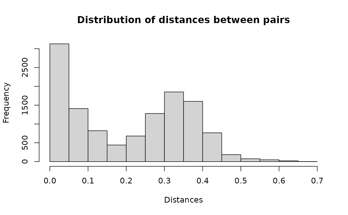
Example pairs.
head(result1$result, n = 10)
#>         x     y block       dist
#>     <int> <int> <num>      <num>
#>  1:     1 12088  8341 0.04520786
#>  2:     2 12156  8379 0.26164961
#>  3:     3  7243  5758 0.04604095
#>  4:     3 10643  5758 0.37306446
#>  5:     4  8422  6453 0.35876358
#>  6:     6  9442  7033 0.31899476
#>  7:     6 10195  7033 0.04166669
#>  8:     7   745   725 0.16333997
#>  9:     8  3072  2772 0.25784391
#> 10:     8 10717  2772 0.12358326
Let’s take a look at the first pair. Obviously there is a typo in the
pername1 but all the other variables are the same, so it
appears to be a match.
cbind(t(census[1, c(1:7, 9:10)]), t(cis[12088, 1:9]))
#>           [,1]              [,2]
#> person_id "SW122AB001001"   "SW122AB001001"
#> pername1  "GEURGE"          "GEORGE"
#> pername2  "HUGHES"          "HUGHES"
#> sex       "M"               "M"
#> dob_day   "19"              "19"
#> dob_mon   "5"               "5"
#> dob_year  "1942"            "1942"
#> enumcap   "1 VICTORIA ROAD" "1 VICTORIA ROAD"
#> enumpc    "SW122AB"         "SW122AB"
Assessing the quality
For some records, we have information about the correct linkage. We can use this information to evaluate our approach.
matches <- merge(x = census[, .(x=1:.N, person_id)],
                 y = cis[, .(y = 1:.N, person_id)],
                 by = "person_id")
matches[, block:=1:.N]
head(matches)
#> Key: <person_id>
#>       person_id     x     y block
#>          <char> <int> <int> <int>
#> 1: DE03US001003  1357 10248     1
#> 2: DE03US008001  4506  2506     2
#> 3: DE03US012002  2706 12005     3
#> 4: DE03US012003  6317 11103     4
#> 5: DE03US013003  4388 10673     5
#> 6: DE03US014003  9463 11793     6
So in our example we have 5991 pairs.
result2 <- blocking(x = census$txt, y = cis$txt, verbose = 1,
                    true_blocks = matches[, .(x, y, block)])
#> ===== creating tokens =====
#> ===== starting search (nnd, x, y: 12671, 12306, t: 1053) =====
#> ===== creating graph =====
Let’s see how our approach handled this problem.
result2
#> ========================================================
#> Blocking based on the nnd method.
#> Number of blocks: 8437.
#> Number of columns used for blocking: 1053.
#> Reduction ratio: 0.9999.
#> ========================================================
#> Distribution of the size of the blocks:
#>    2    3    4    5    6    7    8    9
#> 5559 2100  608  137   26    5    1    1
#> ========================================================
#> Evaluation metrics (standard, in %):
#>      recall   precision         fpr         fnr    accuracy specificity
#>     99.5326     99.7992      0.0000      0.4674     99.9999    100.0000
#>    f1_score
#>     99.6657
It seems that the default parameters of the NND method result in an
FNR of 0.47%. We can see if decreasing the epsilon
parameter as suggested in the Nearest
Neighbor Descent vignette will help.
ann_control_pars <- controls_ann()
ann_control_pars$nnd$epsilon <- 0.2

result3 <- blocking(x = census$txt, y = cis$txt, verbose = 1,
                    true_blocks = matches[, .(x, y, block)],
                    control_ann = ann_control_pars)
#> ===== creating tokens =====
#> ===== starting search (nnd, x, y: 12671, 12306, t: 1053) =====
#> ===== creating graph =====
Changing the epsilon search parameter from 0.1 to 0.2
decreased the FNR to 0.17%.
result3
#> ========================================================
#> Blocking based on the nnd method.
#> Number of blocks: 8447.
#> Number of columns used for blocking: 1053.
#> Reduction ratio: 0.9999.
#> ========================================================
#> Distribution of the size of the blocks:
#>    2    3    4    5    6    7    8    9
#> 5579 2091  606  138   26    5    1    1
#> ========================================================
#> Evaluation metrics (standard, in %):
#>      recall   precision         fpr         fnr    accuracy specificity
#>     99.8331     99.9332      0.0000      0.1669    100.0000    100.0000
#>    f1_score
#>     99.8831
Finally, compare the NND and HNSW algorithm for this example.
result4 <- blocking(x = census$txt, y = cis$txt, verbose = 1,
                    true_blocks = matches[, .(x, y, block)],
                    ann = "hnsw")
#> ===== creating tokens =====
#> ===== starting search (hnsw, x, y: 12671, 12306, t: 1053) =====
#> ===== creating graph =====
It seems that the HNSW algorithm also performed with 0.17% FNR.
result4
#> ========================================================
#> Blocking based on the hnsw method.
#> Number of blocks: 8446.
#> Number of columns used for blocking: 1053.
#> Reduction ratio: 0.9999.
#> ========================================================
#> Distribution of the size of the blocks:
#>    2    3    4    5    6    7    8    9
#> 5586 2078  607  142   26    5    1    1
#> ========================================================
#> Evaluation metrics (standard, in %):
#>      recall   precision         fpr         fnr    accuracy specificity
#>     99.8331     99.9332      0.0000      0.1669    100.0000    100.0000
#>    f1_score
#>     99.8831