Estimate Population Size Using Ratio Regression

Fits the ratio-regression approach for single-source capture-recapture count data as a standalone estimator. The regression is performed on neighbouring marginal-frequency ratios rather than on unit-level counts, which is why this method is separate from the singleRmodels() family framework used by estimatePopsize().

Usage

ratioReg(
  formula,
  data,
  ratioFormula = ~log(k + 1),
  model = c("auto", "M0", "M1"),
  criterion = c("AIC", "BIC"),
  estimator = c("SM", "HT"),
  weights = NULL,
  subset,
  confint = c("bootstrap", "none"),
  B = 1000,
  seed = NULL,
  maxCount = NULL,
  ...
)

Arguments

formula: a formula identifying the observed count column. It must use ~ 1; for example observed ~ 1.
data: a data frame or an object coercible to data.frame.
ratioFormula: a one-sided formula used for the ratio regression on the derived ratio-level data. The default is ~ log(k + 1).
model: which ratio-regression model to use: M0, M1, or auto to select between them by criterion.
criterion: information criterion used when model = "auto".
estimator: which population-size estimator should be treated as the primary one.
weights: optional prior weights interpreted as multiplicities of observed units.
subset: optional logical expression selecting rows from data.
confint: either "bootstrap" for percentile bootstrap intervals or "none" to skip interval estimation.
B: number of bootstrap replicates when confint = "bootstrap".
seed: optional random seed used for bootstrap sampling.
maxCount: optional upper support bound. Counts larger than maxCount are discarded before fitting.
...: additional arguments passed to stats::model.frame().

Value

An object of class singleRRatioReg containing the fitted ratio-regression models, model-selection criteria, derived ratio-level data, observed frequencies, and population-size estimates.

Details

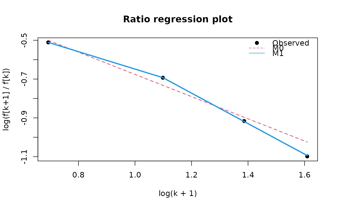
Let \(f_k\) denote the observed frequency of units captured exactly \(k\) times. Ratio regression models the neighbouring ratios \(r_k = f_{k + 1} / f_k\). The default model uses \(\log(r_k) = \beta_0 + \beta_1 \log(k + 1)\) and weighted least squares with weights \(1 / (1 / f_k + 1 / f_{k + 1})\).

Two published models are supported:

M0: ratio regression without one-inflation term
M1: ratio regression with an additional one-inflation indicator I(k == 1)

When model = "auto", both models are fitted and compared by criterion. Population size can then be extracted either through the Horvitz-Thompson (HT) or semi-parametric (SM) estimator, with estimator selecting which one is treated as primary by popSizeEst(), summary(), and plot().

Bootstrap intervals are percentile intervals. For fixed model = "M0" or model = "M1" the bootstrap uses zero-count imputation based on the primary estimator. For model = "auto" it uses the single-bootstrap reselection scheme where model selection is repeated inside each bootstrap sample.

Author

Cyprian Jurkowski, Piotr Chlebicki, Maciej Beręsewicz

Examples

toy_counts <- data.frame(
  observed = c(rep(1, 50), rep(2, 30), rep(3, 15), rep(4, 6), rep(5, 2))
)

toy_fit <- ratioReg(
  observed ~ 1,
  data = toy_counts,
  model = "auto",
  estimator = "SM",
  confint = "none"
)

summary(toy_fit)
#> 
#> Call:
#> ratioReg(formula = observed ~ 1, data = toy_counts, model = "auto", 
#>     estimator = "SM", confint = "none")
#> 
#> Selected ratio regression model: M1 
#> Selection criterion: AIC 
#> Primary population estimator: SM 
#> Observed population size: 103 
#> 
#> Model selection table:
#>    model available logLik     AIC    BIC selected
#> M0    M0      TRUE   7.85  -9.701 -11.54    FALSE
#> M1    M1      TRUE  20.14 -32.284 -34.74     TRUE
#> 
#> Coefficients for M0 :
#> (Intercept)  log(k + 1) 
#>     -0.1035     -0.5724 
#> 
#> Coefficients for M1 :
#>  (Intercept)   log(k + 1) oneInflation 
#>       0.1714      -0.7865      -0.1371 
#> 
#> Population size estimates:
#>  estimator pointEstimate variance lowerBound upperBound
#>         HT      139.7316       NA         NA         NA
#>         SM      139.7308       NA         NA         NA
popSizeEst(toy_fit)
#> Point estimate: 139.7308
#> Variance: NA
#> 95% confidence intervals:
#>   lowerBound upperBound
#> 1         NA         NA
plot(toy_fit)


toy_tab <- aggregate(list(weight = rep(1, nrow(toy_counts))),
                     by = list(observed = toy_counts$observed),
                     FUN = sum)
ratioReg(
  observed ~ 1,
  data = toy_tab,
  weights = toy_tab$weight,
  model = "M0",
  confint = "none"
)
#> Call: ratioReg(formula = observed ~ 1, data = toy_tab, model = "M0", 
#>     weights = toy_tab$weight, confint = "none")
#> 
#> Selected ratio regression model: M0 
#> Selection criterion: AIC 
#> Primary population estimator: SM 
#> Observed population size: 103 
#> 
#> Coefficients:
#> (Intercept)  log(k + 1) 
#>  -0.1035021  -0.5723849 
#> 
#> Population size estimation results:
#> Point estimate: 157.869
#> Variance: NA
#> 95% confidence intervals:
#>   lowerBound upperBound
#> 1         NA         NA
#> 
#> Alternative estimator point estimate: HT = 158.467